P36
Linear Solver
Many numerical problems are ended up with solving a linear system:
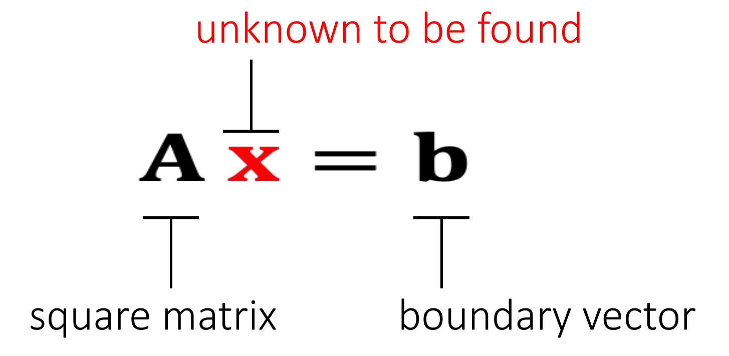
It's expensive to compute \(\mathbf{A^{-1}} \), especially if \(\mathbf{A} \) is large and sparse. So we cannot simply do:\(\mathbf{x = A^{-1}b}\).
- 当 \(\mathbf{A}\) 是稀疏时. \(\mathbf{A}^{-1}\)通常不是稀疏。 如果 \(\mathbf{A}\) 很大,\(\mathbf{A}^{-1}\)会占用大量空间。
- 计算\(\mathbf{A}^{-1}\)非常耗时
P25
An Incomplete Summary
There are two popular linear solver approaches: direct and iterative.
-
Direct Solvers (LU, LDLT, Cholesky, Intel MKL PARDISO)
- One shot, expensive but worthy if you need exact solutions.
- Little restriction on \(\mathbf{A}\)
- Mostly suitable on CPUs
-
Iterative Solvers( Jacobbi. Gauss-Seidel,共轭梯度)
- Expensive to solve exactly, but controllable
- Convergence restriction on \(\mathbf{A}\), typically positive definiteness
- Suitable on both CPUs and GPUs
- Easy to implement
- Accelerable: Chebyshev, Nesterov, Conjugate Gradient
P37
Direct Linear Solver
方法
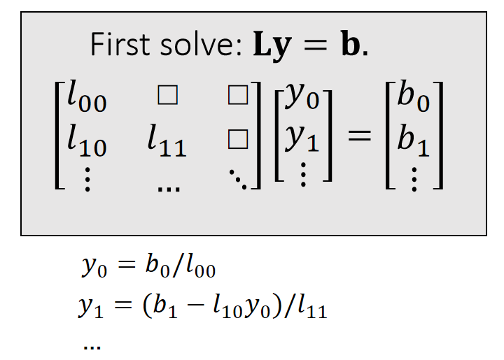
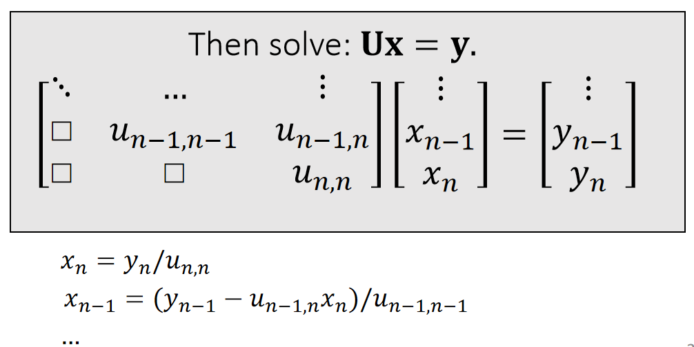
A direct solver is typically based LU factorization, or its variant: Cholesky, \(\mathrm{LDL^\top } \), etc…
✅ \(\mathbf{LU}\) 可用于非对称矩阵。
Cholesky 和 \( \mathbf{LDL^\top}\) 仅用于对称矩阵,但内存消耗更少。
这里不介绍如何做\(\mathbf{LU}\)分解
$$ \mathbf{A=LU=} \begin{bmatrix} l_{00} & \Box & \Box \\ l_{10} & l_{11} & \Box \\ \vdots & \cdots &\ddots \end{bmatrix}\begin{bmatrix} \ddots & \cdots &\vdots \\ \Box&u_{n−1,n−1} &u_{n−1,n} \\ \Box & \Box &u_{n,n} \end{bmatrix} $$ \(\quad\quad\quad\quad\quad\quad\quad\)lower triangular \(\quad\quad\) upper triangular
P38
分析
- When \(\mathbf{A}\) is sparse, \(\mathbf{L}\) and \(\mathbf{U}\) are not so sparse. Their sparsity depends on the permutation.(See matlab)
✅ \(\mathbf{L}、\mathbf{U}\) 和稀疏性与行列顺序有关,因此通常在\(\mathbf{LU}\) 分解之前做 permutation,使得到比较好的顺序。
- lt contains two steps: factorization and solving. lf we must solve many linear systems with the same \(\mathbf{A}\) , we can factorize it only once.
✅ \(\mathbf{LU}\) 分解是计算量的大头,只做一次 \(\mathbf{LU}\) 分解,能省去大量计算。
- Cannot be easily parallelized:Intel MKL PARDISO
P39
Iterative Linear Solver
An iterative solver has the form:
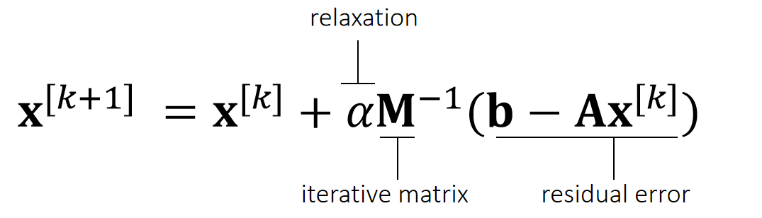
Why does it work?
$$ \begin{matrix} \mathbf{b−Ax} ^{[k+1]} =\mathbf{b−Ax} ^{[k]}−\mathbf{αAM} ^{−1}(\mathbf{b−Ax} ^{[k]}) \\ \quad\quad\quad\quad\quad\quad\quad\quad\quad\quad=(\mathbf{I−αAM} ^{−1})(\mathbf{b−Ax} ^{[k]}) =(\mathbf{I−αAM} ^{−1})^{k+1}(\mathbf{b−Ax} ^ {[0]}) \end{matrix} $$
So,
\(\mathbf{b−Ax} ^{[k+1]}→0\), if \(ρ(\mathbf{I−αAM} ^{−1})<1.\)
✅\(\mathbf{b-Ax}^{[k+1]}\) 代表下一时的残差,迭代要想收敛,\(\mathbf{b-Ax}^{[k+1]}\) 应趋于0
\(\rho\):矩阵的spectral radius (the largest absolute value of the eigenvalues)
✅ 不会真的去算 \(\rho\),而是调\(α\),试错。 因为求特征值的代价比较大
P40
\(\mathbf{M}\) must be easier to solve:
| \(\mathbf{M} =\mathrm{diag} (\mathbf{A} )\) Jacobi Method |
|---|
\(\quad\)
| \(\mathbf{M} =\mathrm{lower} (\mathbf{A} )\) Gauss-Seidel Method |
|---|
The convergence can be accelerated: Chebyshev, Conjugate Gradient, … (Omitted here.)
优点:
- simple
- fast for inexact solution
- paralleable
缺点:
- convergence condition
✅ 例如要求M是正定的或对角占优的
- slow for exact solution
P24
The Jacobi Method
We can use the Jacobi method to solve \(\mathbf{A}∆\mathbf{x} = \mathbf{b} \).
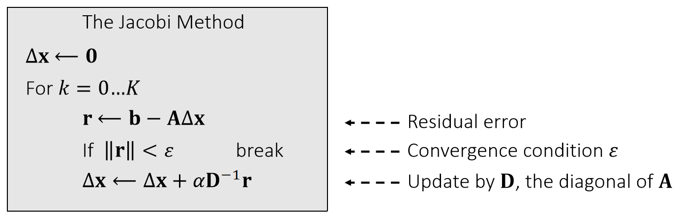
The vanilla Jacobi method (\(α\) = 1) has a tight convergence requirement on \(\mathbf{A}\), i.e., being diagonal dominant.
The use of \(α\) allows the method to converget even when \(\mathbf{A}\) is positive definite only.
P26
The Jacobi Method with Chebyshev Acceleration
We can use the accelerated Jacobi method to solve \(\mathbf{A}∆\mathbf{x} =\mathbf{b} \).
The Accelerated Jacobi Method
\(∆\mathbf{x} \longleftarrow \mathbf{0} \)
last_\(∆\mathbf{x} \longleftarrow \mathbf{0}\)
For \(k=0\dots \mathbf{K}\)
\(\mathbf{r} \longleftarrow \mathbf{b} −\mathbf{A} ∆\mathbf{x}\)
If \(||\mathbf{r} ||<\omega \quad\) break
If \(k=0 \quad\quad\quad \omega =1\)
Else If \( k=1 \quad \quad\quad\omega =2/(2-\rho^2)\)
Else \(\quad\quad\quad\omega =4/(4-\rho ^2\omega )\)
old_\(∆ \mathbf{x} \longleftarrow ∆ \mathbf{x}\)
\(∆\mathbf{x} ⟵∆\mathbf{x} +\mathbf{αD} ^{−1}\mathbf{r}\)
\(∆\mathbf{x} \longleftarrow \omega ∆ \mathbf{x} +(1−\omega)\)last_∆\(\mathbf{x}
\)
last_\(∆\mathbf{x} \longleftarrow \) old_\(∆\mathbf{x}\)
\(\rho (\rho <1)\) is the estimated spectral radius of the iterative matrix.
课后答疑
问题二:怎么加速?
答:用 Jacobian 可以在 GPU 上加速、直接法比迭代法慢。
问题三:共轭梯度
共轭梯度的效率很大程度上取决于 precondition,但在GPU上能使用的precondition 比较受限、 CPU 上一般选择 Incomplete LU 分解。
问题四:支持的维度
直接法比较占内存,因此支持的维度不如迭代法大。
本文出自CaterpillarStudyGroup,转载请注明出处。
https://caterpillarstudygroup.github.io/GAMES103_mdbook/