P3
A Grid Representation and Finite Differencing
P4
A Regular Grid Representation
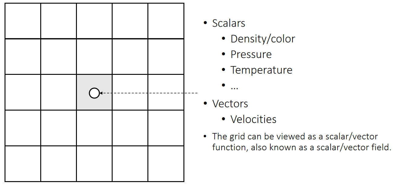
✅ 把场定义在标准格子上的好处:(1)把物理量定义在格子的中心(2)计算导数或利用导数进行微分计算变得容易了。
✅ 上节课grid用1D来表示2D,2D表示3D,不是真正的grid方法。
🔎 Central Differencing:L10.
✅ 空间中任意位置的物理量由格子中心插值得出。
P6
Finite Differencing on Grid
P13
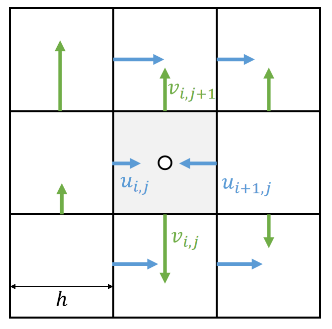
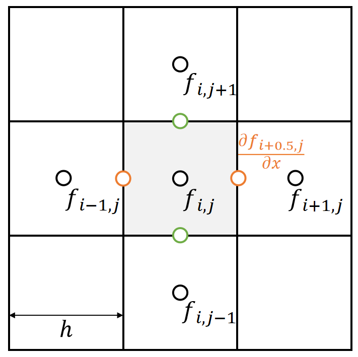
Staggered Grid 表示
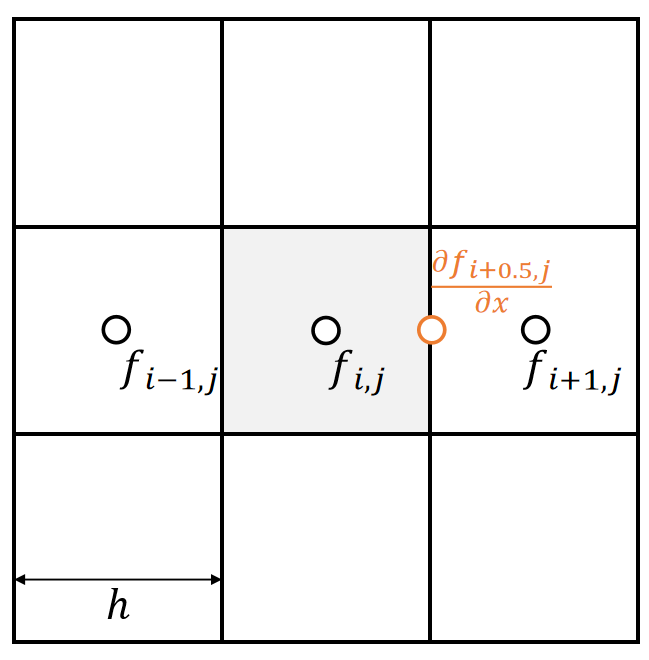
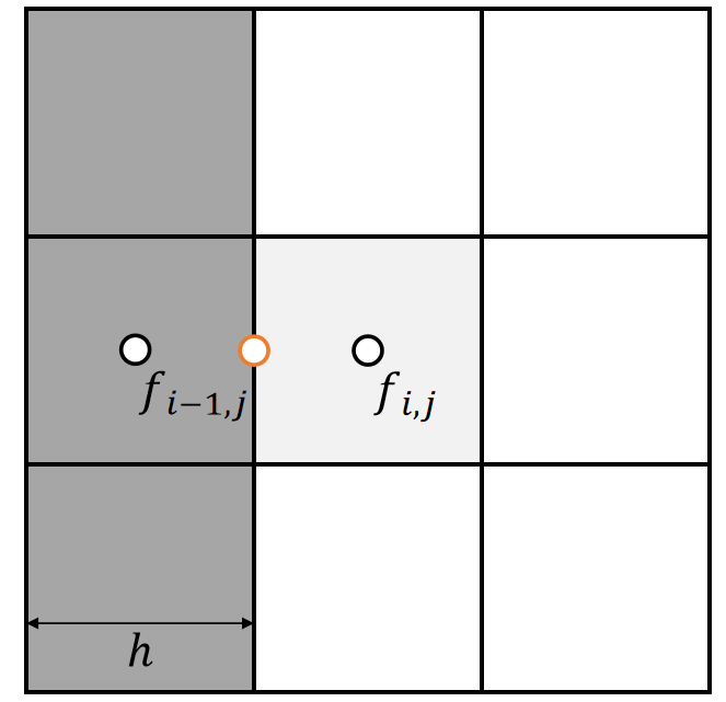
Problem with Regular Grid 表示
Central differencing gives the derivative in the middle.
-
The cell doesn’t exist at (i+0.5, j).
-
To get \( \frac{∂f_ {i,j}}{∂x} \), we need \(f_{i−1,j}\) and \(f_{i+1,j}\). But this is weird, because \(f_{i,j}\) is unused.
✅ 前面假设所有物理量定义在格子的中间。但此处算出来的一阶微分量不在格子中间。
P14
Solution: 把速度属性放在墙上
✅ 不规定所有物理量都定义在格子中间,也可以定义在墙上。
✅ 对照 Height Fleld 方法,也是把 \(P\) 和 \(H\) 定义在格子上,把速度定义在格子交界处。
We define some physical quantities on faces, specifically velocities.
-
The x-part of the velocity is defined on vertical faces.
-
The y-part of the velocity is defined on horizonal faces.
✅ 把速度定义在墙上的好处量,速度是矢量、可以用不同方向的墙表达不同方向上的速度、直观。
The grid is very friendly with central differencing.
一阶导数
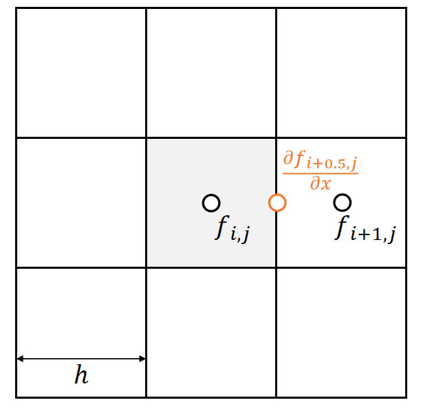
| $$\frac{∂f_{i+0.5,j}}{∂x}≈\frac{f_{i+1,j}−f_{i,j}}{ℎ}$$ |
|---|
P7
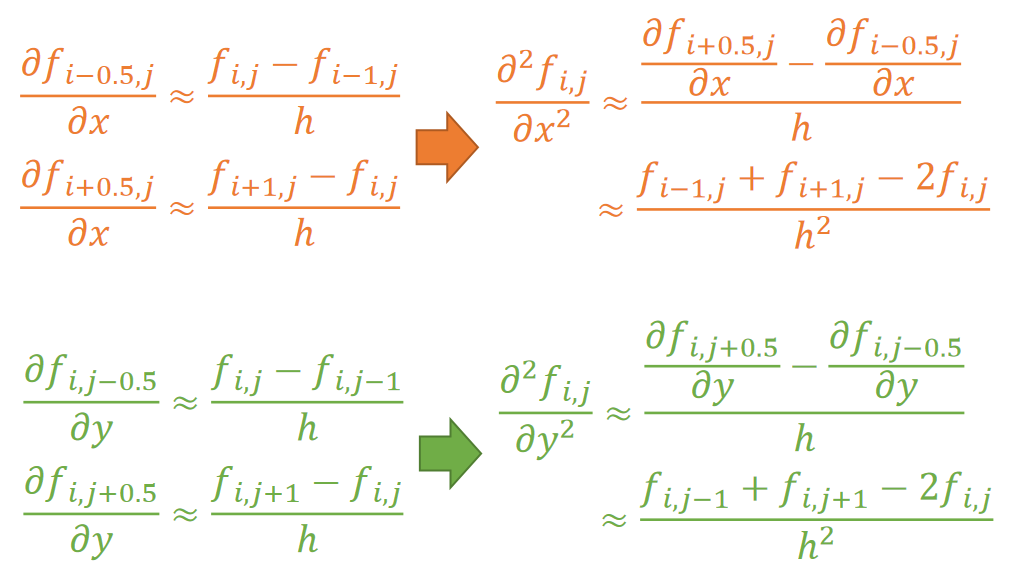
二阶导数
P8
Discretized Laplacian
We can then obtain the discretized Laplacian operator on grid.
$$ \frac{∂^2f_{i,j}}{∂x^2}≈\frac{\frac{∂f_{i−0.5,j}}{∂x}−\frac{∂f_{i+0.5,j}}{∂x}}{ℎ}≈\frac{f_{i−1,j}+f_{i+1,j}−2f_{i,j}}{ℎ^2} $$
$$ \frac{∂^2f_{i,j}}{∂y^2}≈\frac{\frac{∂f_{i,j+0.5}}{∂y}−\frac{∂f_{i,j−0.5}}{∂y}}{ℎ} ≈\frac{f_{i,j−1}+f_{i,j+1}−2f_{i,j}}{ℎ^2} $$
| $$∆f_{i,j}=\frac{∂^2f_{i,j}}{∂x^2}+\frac{∂^2f_{i,j}}{∂y^2}≈\frac{f_{i−1,j}+f_{i+1,j}+f_{i,j−1}+f_{i,j+1−4}f_{i,j}}{ℎ^2} $$ |
|---|
✅ 网格上的Laplace算子。
P9
Boundary Conditions
The boundary condition specifies \(f_{i−1,j}\) if it’s outside.
A Dirichlet boundary: \(f_{i−1,j}=C\)
| $$ ∆f_{i,j}≈\frac{C+f_{i+1,j}+f_{i,j−1}+f_{i,j+1}−4f_{i,j}}{ℎ^2}$$ |
|---|
A Neumann boundary: \(f_{i−1,j}=f_{i,j}\)
| $$∆f_ {i,j} ≈ \frac{f_ {i+1,j}+f_ {i,j−1}+f_ {i,j+1}−3f_{i,j}}{ℎ^2}$$ |
|---|
✅ 至少有一个边界使用Dirithlet.否则会全部收缩为0.
✅ Neumann是约束相对关系,没有绝对数值,会有无穷多解。
本文出自CaterpillarStudyGroup,转载请注明出处。
https://caterpillarstudygroup.github.io/GAMES103_mdbook/