P22

Projective Dynamics

原理

Instead of blending projections in a Jacobi or Gauss-Seidel fashion as in PBD, projective dynamics uses projection to define a quadratic energy.

✅ PBD方法直接拿约束来修复顶点位置，没有物理含义。而本页方法把projection方法跟物拟模拟结合起来，主要体现在用约束来做什么。

能量和力

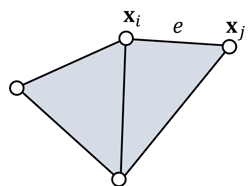
$E(\mathbf{x} ) = {\textstyle \sum_{e = (i,j)}}\frac{1}{2} ||(\mathbf{x} _i−\mathbf{x} _j)−(\mathbf{x} _{e,i}^{\mathrm{new} }−\mathbf{x} _{e,j}^{\mathrm{new} })||^2$

{$\mathbf{x} _{e,i}^{\mathrm{new} },\mathbf{x} _{e,j}^{\mathrm{new} }$} = $\mathrm{Projection} _e(\mathbf{x}_i,\mathbf{x}_j)$ for every edge $e$

✅ 本文基于约束定义能量。{$\mathbf{x} _{e,i}^{\mathrm{new} },\mathbf{x} _{e,j}^{\mathrm{new} }$}为期望的顶点位置。不直接把顶点从当前位置移到期望位置。而是把当前位置和期望位置的距离转化为能量，通过能量推动顶点从当前位置移到目标位置。

$$E(\mathbf{x})=\sum _{e=(i,j)}\frac{k}{2}(||\mathbf{x}_i-\mathbf{x}_j||-L_e)^2$$

$$\mathbf{f} _i=−\nabla_iE(\mathbf{x} )=−{\textstyle \sum _{e:i\in e}}(\mathbf{x} _i−\mathbf{x} _j)−(\mathbf{x} _{e,i}^{\mathrm{new}} −\mathbf{x} _{e,j}^{\mathrm{new} })$$

✅ 基于 $E(\mathbf{x})、\mathbf{x}_i^{\mathrm{new} } 、\mathbf{x}_j^{\mathrm{new} }$ 计算力，此时假设$\mathbf{x}_i^{\mathrm{new} }$和 $\mathbf{x}_j^{\mathrm{new} }$都是定值，$\mathbf{x}_i$和 $\mathbf{x}_j$是变量。
✅ 本文基于约束定义能量和力，得到的结果与基于弹簧能量计算的能量和力相同。
✅ 既然 $E$ 和 $F$ 是一样的，何必多此一举? 答：H不同。

P23

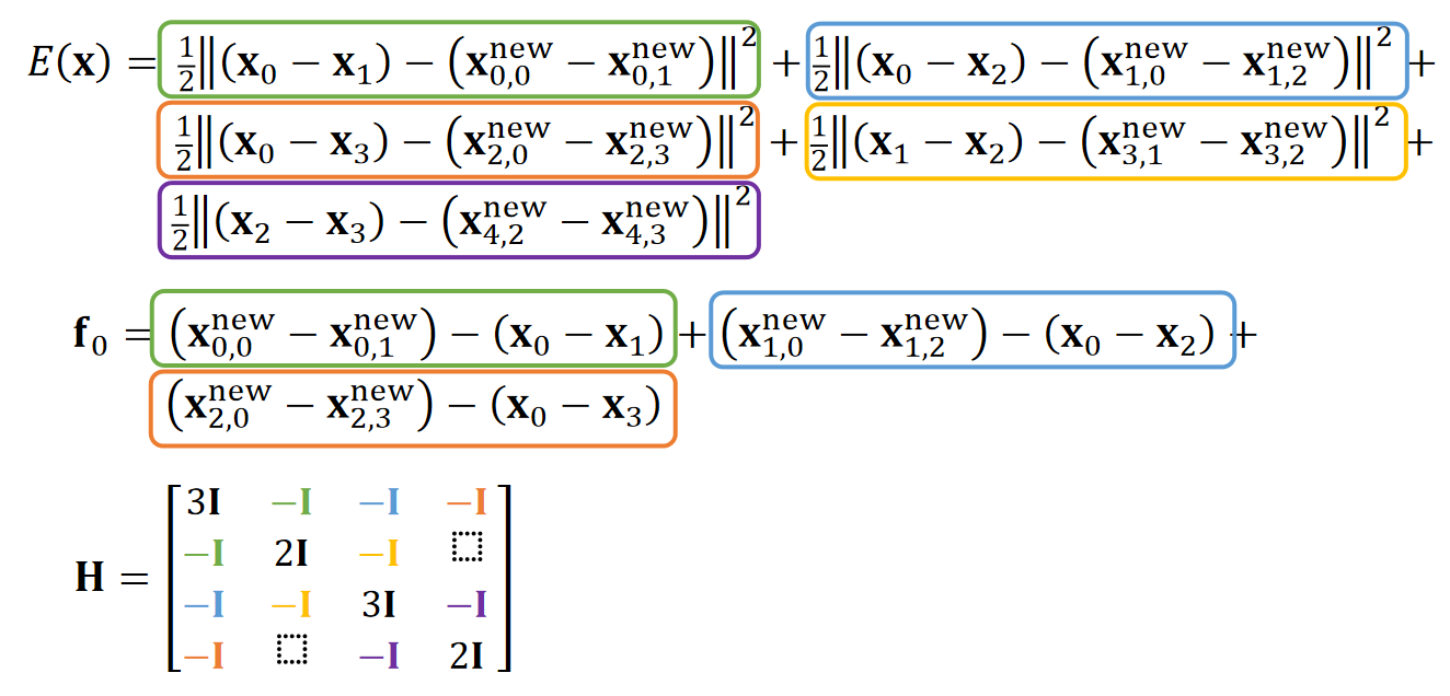
Hessian 矩阵

Instead of blending projections in a Jacobi or Gauss-Seidel fashion as in PBD, projective dynamics uses projection to define a quadratic energy.

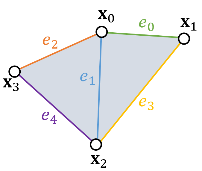
✅ 同一个顶点在三个不同边上的投影是不同的。
✅ 可以直接根据Mesh的拓扑关系构造H矩阵。
✅ 为什么能简化$\mathbf{H}$的计算？答：在计算某一个端点时，假设另一个端点不动（常量），那么能量就是只关于这个端点的二次函数

P24

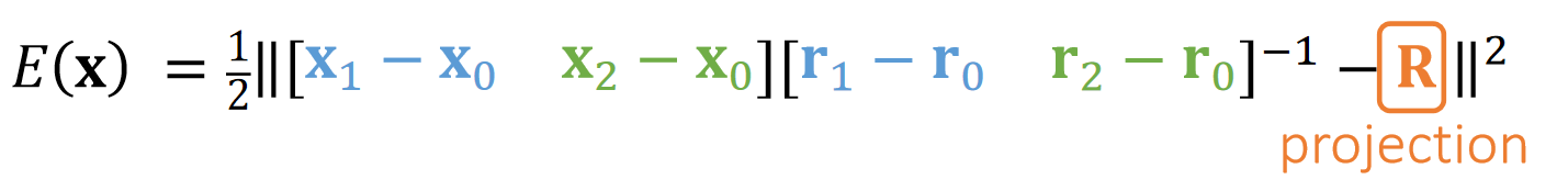
Shape Matching

Shape matching is also projective dynamics, if we view rotation as projection:

|

The 2D Space	The 3D Space

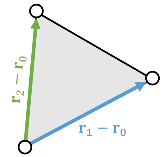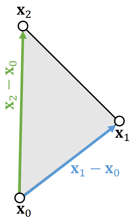Assuming that $\mathbf{{\color{Orange} R} }$ is constant,
$$\begin{matrix} \mathbf{f} _0=−\nabla_0E(\mathbf{x} )\\ \mathbf{f} _1=−\nabla_1E(\mathbf{x} ) \\ \mathbf{f} _2=−\nabla_2E(\mathbf{x} )\\ \mathbf{H} =\frac{∂E^2(\mathbf{x} )}{∂x^2} \quad \text{is a constant !} \end{matrix}$$

P25

Simulation by Projective Dynamics

• According to implicit integration and Newton’s method, a projective dynamics simulator looks as follows, with matrix $\mathbf{A} =\frac{1}{∆t^2}\mathbf{M+}\mathbf{H}$ being constant.

• We can use a direct solver with only one factorization of A.

✅ 解线性系统的主要耗时在LU分解，而这个算法中$\mathrm{H}$是常数矩阵，只需要做一次LU分解，简化了对$\mathrm{H}$分解的计算量。

Initialize $\mathbf{x} ^{(0)}$, often as$\mathbf{x} ^{[0]}$or $\mathbf{x} ^{[0]} +∆t\mathbf{v} ^{[0]}$

For $k=0\dots K$
$\quad$ Recalculate projection

✅ 对于弹簧系统，Recaculate projection 这一步实际上不需要，因为直接用弹簧系统的公式算力，得到的$f$是一样的。
✅ 如果是做 shape matching, 还是需要这一步，用于算 $f$

$\quad$ Solve $(\frac{1}{∆t^2}\mathbf{M} +\mathbf{H} )∆\mathbf{x} =−\frac{1}{∆t^2}\mathbf{M} (\mathbf{x} ^{(k)}−\mathbf{x} ^{[0]}−∆t\mathbf{v} ^{[0]})+\mathbf{f} (\mathbf{x} ^{(k)})$

$\quad$ $\mathbf{x} ^{(k+1)}\longleftarrow \mathbf{x} ^{(k)}+∆\mathbf{x}$

$\quad$ If $||∆\mathbf{x}||$ is small $\quad$ then break

$\mathbf{x} ^{[1]}\longleftarrow \mathbf{x} ^{(k+1)}$

$\mathbf{v} ^{[1]}\longleftarrow (\mathbf{x} ^{[1]}-\mathbf{x} ^{[0]})/∆t$

“Newton’s Method”

$$\quad$$

P26

Preconditioned Steepest Descent

• Mathematically, this approach is preconditioned steepest descent, in which:

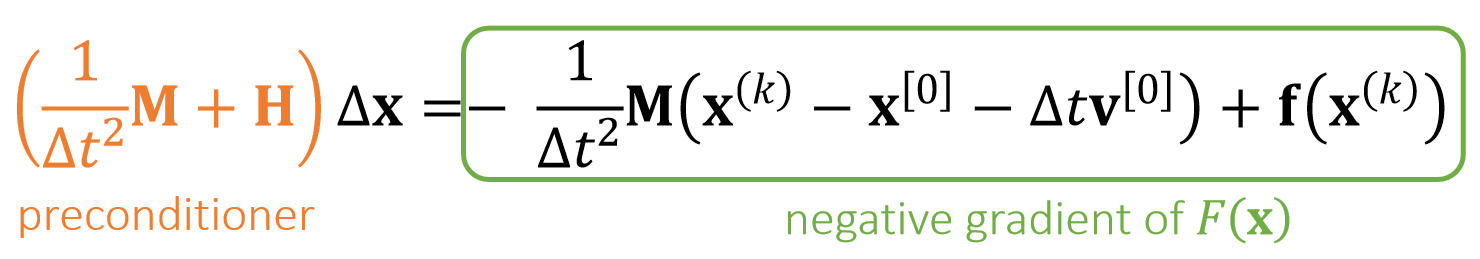
$$F(\mathbf{x} )=\frac{1}{2∆t^2} ||\mathbf{x} −\mathbf{x} ^{[0]}−∆t\mathbf{v} ^{[0]}||_\mathbf{M} ^2+E(\mathbf{x} )$$

The performance depends on how well $\mathbf{{\color{Orange} H} }$ approximates the real Hessian.

✅$\mathrm{H}$不需要很精确，一个近似的正定的矩阵，就能让结果收敛。

P27

Pros and Cons of Projective Dynamics

• By building constraints into energy, the simulation now has a theoretical solution with physical meaning.
• Fast on CPUs with a direct solver. No more factorization!

✅ Fast on CPU,因为它只作一次$\mathbf{LU}$分解。

• Fast convergence in the first few iterations.
• Slow on GPUs. (GPUs don’t support direct solver wells.)

✅ Slow on GPU，因为$\mathbf{LU}$分解不适用于 $\mathbf{GPU}$

• Slow convergence over time, as it fails to consider Hessian caused by projection.
  • Still suffering from high stiffness
• Cannot easily handle constraint changes.

✅ constraint changes: 网格关系改变导至弹簧结构改变，原来的$\mathbf{H}$将不再适用。
- Contacts
- Remeshing due to fracture, etc.

✅ 课后答疑：
能量优化的方法很少用于刚体，主要是有限元、弹性体、衣服模拟。

P28

After-Class Reading

Bouaziz et al. 2014. Projective Dynamics: Fusing Constraint Projections for Fast Simulation. TOG (SIGGRAPH).

本文出自CaterpillarStudyGroup，转载请注明出处。

https://caterpillarstudygroup.github.io/GAMES103_mdbook/