P26

Matrix: Basics

Matrix: Definition

A real matrix is a set of real elements arranged in rows and columns.

$$A=\begin{bmatrix} a_{00} & a_{01} & a_{02} \\ a_{10}& a_{11} & a_{12} \\ a_{20}& a_{21} & a_{22} \end{bmatrix}=[a_{0} \quad a_{1} \quad a_{2}]\in \mathbf{R} ^{3\times 3}$$

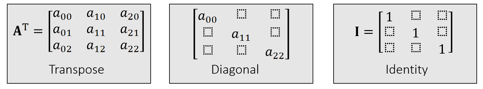
$$\mathbf{A^T=A} \quad \mathrm{Symmetric}$$

P27

Matrix: Multiplication

How to do matrix-vector and matrix-matrix multiplication? (Omitted)

• $\mathbf{AB≠BA} \quad \quad \quad \quad \quad \quad \quad \quad \mathbf{(AB)x=A(Bx)}$
• $\mathbf{(AB)^T=B^TA^T} \quad \quad \quad \quad \quad \quad \mathbf{(A^TA)^T=A^TA}$
• $\mathbf{Ix=x} \quad \quad \quad \quad \quad \quad \quad \quad \quad \mathbf{AI=IA=A}$
  $\quad$
• $\mathbf{A^{−1}:  AA^{−1}=A^{−1}A=I} \quad \quad \mathrm{inverse}$
• $\mathbf{(AB)^{−1}=B^{−1}A^{−1}}$
• Not every matrix is invertible, e.g., $\mathbf{A} =\begin{bmatrix} 0 & 0 & 0\\ 0 & 0 & 0\\ 0 & 0 & 0 \end{bmatrix}$

P28

Matrix: Orthogonality

An orthogonal matrix is a matrix made of orthogonal unit vectors.

$$\mathbf{A} =[\mathbf{a} _0\quad \mathbf{a} _1\quad \mathbf{a} _2]\quad\mathrm{such \quad that } \quad \mathbf{a}_i^\mathbf{T}\mathbf{a}_j =\begin{cases} 1，& \text{ if } i= j \text{(unit)}\\ 0.& \text{ if } i\ne j \text{(orthogonal)} \end{cases}$$

$$\mathbf{A^TA}=\begin{bmatrix} \mathbf{a}_0^\mathbf{T} \\ \mathbf{a}_1^\mathbf{T} \\ \mathbf{a}_2^\mathbf{T} \end{bmatrix}\begin{bmatrix} \mathbf{a}_0 & \mathbf{a}_1 &\mathbf{a}_2 \end{bmatrix}=\begin{bmatrix} \mathbf{a}_0^\mathbf{T} \mathbf{a}_0 & \mathbf{a}_0^\mathbf{T} \mathbf{a}_1 & \mathbf{a}_0^\mathbf{T} \mathbf{a}_2\\ \mathbf{a}_1^\mathbf{T} \mathbf{a}_0 & \mathbf{a}_1^\mathbf{T} \mathbf{a}_1 & \mathbf{a}_1^\mathbf{T} \mathbf{a}_2\\ \mathbf{a}_2^\mathbf{T} \mathbf{a}_0 & \mathbf{a}_2^\mathbf{T} \mathbf{a}_1 & \mathbf{a}_2^\mathbf{T} \mathbf{a}_2 \end{bmatrix}=I$$

$$\mathbf{A^T=A^{-1}}$$

P29

Matrix Transformation

A rotation can be represented by an orthogonal matrix.

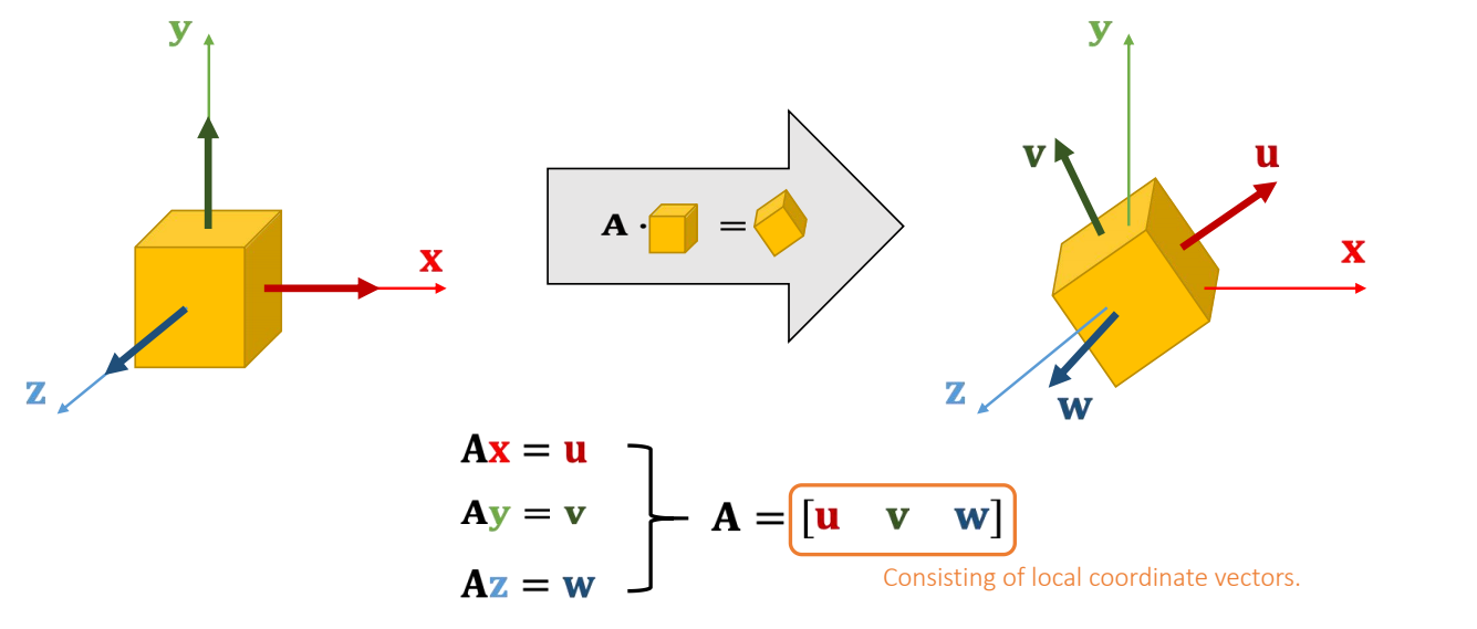
✅ $\mathbf{x、y、z}$ 是世界坐标系、 $\mathbf{u、v、w}$ 是局部坐标系，旋转矩阵是局部坐标系在世界坐标系中的状态的描述。

P30
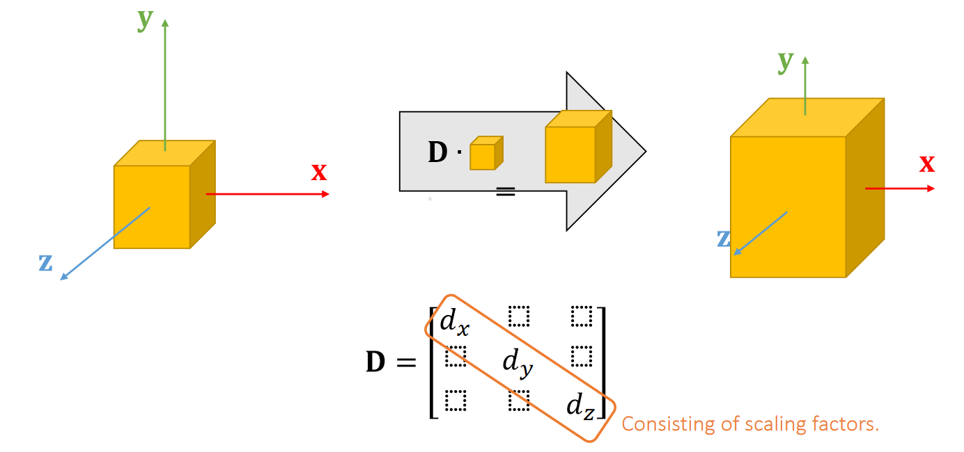
A scaling can be represented by a diagonal matrix.

P31

矩阵分解

Singular Value Decomposition

A matrix can be decomposed into:
$\mathbf{A=UDV^T} \quad$such that $\mathbf {D}$ is diagonal,and $\mathbf {U}$ and $\mathbf {V}$ are orthogonal.
$\quad \quad \quad \quad\quad$ D 的对角线元素是singular values（奇异值）

Any linear deformation can be decomposed into three steps: rotation, scaling and rotation:

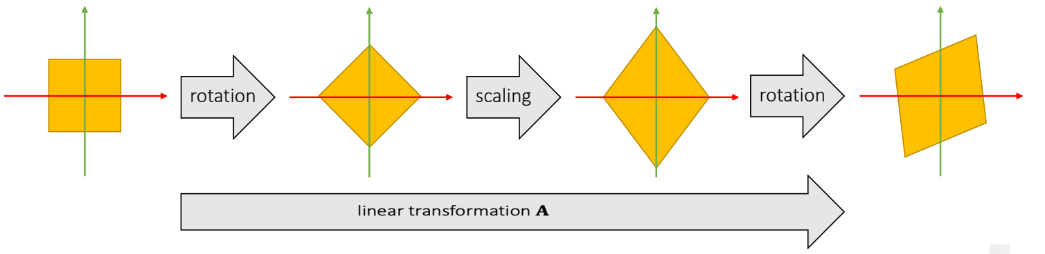
✅ rotation $\longrightarrow$ scaling $\longrightarrow$ rotation 分别对应 $\mathbf{V}_2^\mathbf{T},\mathbf{D}, \mathbf{U}$. 注意顺序！！！
所有 $\mathbf{A}$ 都能做 $\mathbf{SVD}$

P32

Eigenvalue Decomposition

A symmetric matrix can be decomposed into:
$\mathbf{A=UDU^{-1}}\quad$such that $\mathbf {D}$ is diagonal,and $\mathbf {U}$ is orthogonal.
$\quad \quad \quad \quad\quad$ D 的对角线元素是eigenvalues（特征值）

✅ $\mathbf{ED}$ 看作是$\mathbf{SVD}$的特例，仅应用于对称矩阵，此时 $\mathbf{U=V}$
$\mathbf{U}$ 是正交矩阵，因此也可写成 $\mathbf{A = UVU^T}$

As in the textbook
Let $\mathbf{U} =\begin{bmatrix} \cdots & \mathbf{u} _i &\cdots \end{bmatrix}$, we have:
$$\mathbf{Au} _i= \mathbf{UDU^T} \mathbf{u} _i=\mathbf{UD} \begin{bmatrix} \vdots \\ 0\\ 1\\ 0\\ \vdots \end{bmatrix}=\mathbf{U} \begin{bmatrix} \vdots \\ 0\\ d_i\\ 0\\ \vdots \end{bmatrix}=d_i\mathbf{u} _i$$ $\mathbf{U}$: 是 the eigenvector of $d_i$
$d_i$: 是 eigenualue

We can apply eigenvalue decomposition to asymmetric matrices too, if we allow eigenvalues and eigenvectors to be complex. Not considered here.

✅ complex：复数
图形学不考虑虚数，因此也不考虑非对称矩阵的 $\mathbf{ED}$

P33

Symmetric Positive Definiteness (s.p.d.)

定义

$\mathbf{A}$ is s.p.d. if only if: $\quad\quad\quad\quad\quad\quad\quad\quad$ $\mathbf{v^TAv}>0$, for any $\mathbf{v} ≠ 0.$

$\mathbf{A}$ is symmetric semi-definite if only if: $\quad\quad$ $\mathbf{v^TAv}≥0$, for any $\mathbf{v}≠ 0$.

✅ 计算矩阵的有限元或 Hession 时会用到正定性

怎么理解SPD

$d>0 \quad\quad\quad\quad\Leftrightarrow \quad \mathbf{v^T} d\mathbf{v} >0$, for any $\mathbf{v} ≠ 0.$

$d_0, d_1,…>0 \quad\Leftrightarrow \quad \mathbf{v^TDv=v^T} \begin{bmatrix} \ddots & \Box & \Box\\ \Box & d_i & \Box\\ \Box &\Box &\ddots \end{bmatrix}\mathbf{v} >0$, for any $\mathbf{v} ≠0.$

✅ 一堆大于零的实数组成一个对角矩阵, 公式1的扩展

$d_0, d_1,…>0  \quad\Leftrightarrow \quad \mathbf{v^T(UDU^T)v=v^TUU^T(UDU^T)UU^Tv}$

$\mathbf{U}$ orthogonal $\quad\quad\quad\quad\quad\quad\quad\quad=\mathbf{(U^Tv)^T(D)(U^Tv)>0 }$, for any $\mathbf{v} ≠0$

✅ 公式3是公式2的扩展

P34

怎么判断SPD

• A is s.p.d. if only if all of its eigenvalues are positive:
  $\mathbf{A=UDU^T}$ and $d_o,d_1,\cdots > 0.$

• But eigenvalue decomposition is a stupid idea most of the time, since it takes lotsof time to compute.

✅ 实际上不会通过 $\mathbf{ED}$ 来判断矩阵的正定性。因为ED的计算量很大。

• In practice, people often choose other ways to check if A is sp.d. For example,

$a_{ii}>∑_{i≠j}|a_{ij}|$ for all $i$
A diagonally dominant matrix is p.d.

$$\begin{bmatrix} 4&3 & 0\\ -1& 5 &3 \\ -8& 0 &9 \end{bmatrix}\begin{matrix}\quad\quad \quad4>3+0\\ \quad\quad\quad 5>1+3 \\ \quad\quad9>8 \end{matrix}$$

✅ 对角占优矩阵必定正定，正定不一定对角占优

• Finally, a s.p.d.matrix must be invertible:
  $$\mathbf{A^{-1} =(U^T)^{-1}D^{-1}U^{-1} = UD^{-1}U^T}.$$

P35

例子

Prove that if A is s.p.d., then $\mathbf{B} =\begin{bmatrix} \mathbf{A} &\mathbf{-A} \\ \mathbf{-A} &\mathbf{A} \end{bmatrix}$is symmetric semi-definite.

For any $\mathbf{x}$ and $\mathbf{y}$, we know:

$$\begin{bmatrix} \mathbf{ x^T}&\mathbf{ y^T} \end{bmatrix}\mathbf{B}\begin{bmatrix} \mathbf{x} \\ \mathbf{y} \end{bmatrix}=\begin{bmatrix} \mathbf{ x^T}&\mathbf{ y^T} \end{bmatrix}\begin{bmatrix} \mathbf{A} &\mathbf{-A} \\ \mathbf{-A} &\mathbf{A} \end{bmatrix}\begin{bmatrix} \mathbf{x} \\ \mathbf{y} \end{bmatrix}$$

$$\quad\quad\quad\quad\quad\quad\quad\quad\quad\quad\mathbf{=x^TA(x-y)-y^TA(x-y)=(x-y)^TA(x-y)}$$

Since A is sp.d., we must have:

$$\begin{bmatrix} \mathbf{ x^T} & \mathbf{y^T} \end{bmatrix}\mathbf{B} \begin{bmatrix} \mathbf{x} \\ \mathbf{y} \end{bmatrix}\ge 0$$

P36

Linear Solver

Many numerical problems are ended up with solving a linear system:

It's expensive to compute $\mathbf{A^{-1}}$, especially if $\mathbf{A}$ is large and sparse. So we cannot simply do:$\mathbf{x = A^{-1}b}$.

There are two popular linear solver approaches: direct and iterative.

✅ 当 $\mathbf{A}$ 是稀疏时. $\mathbf{A}^{-1}$通常不是稀疏。 如果 $\mathbf{A}$ 很大， $\mathbf{A}^{-1}$会占用大量空间

P37

Direct Linear Solver

方法

A direct solver is typically based LU factorization, or its variant: Cholesky, $\mathrm{LDL^\top }$, etc…

✅ $\mathbf{LU}$ 可用于非对称矩阵。
Cholesky 和 $\mathbf{LDL^\top}$ 仅用于对称矩阵，但内存消耗更少。
这里不介绍如何做$\mathbf{LU}$分解

$$\mathbf{A=LU=} \begin{bmatrix} l_{00} & \Box & \Box \\ l_{10} & l_{11} & \Box \\ \vdots & \cdots &\ddots \end{bmatrix}\begin{bmatrix} \ddots & \cdots &\vdots \\ \Box&u_{n−1,n−1} &u_{n−1,n} \\ \Box & \Box &u_{n,n} \end{bmatrix}$$ $\quad\quad\quad\quad\quad\quad\quad$lower triangular $\quad\quad$ upper triangular

P38

分析

• When $\mathbf{A}$ is sparse, $\mathbf{L}$ and $\mathbf{U}$ are not so sparse. Their sparsity depends on the permutation.(See matlab)

✅ $\mathbf{L}、\mathbf{U}$ 和稀疏性与行列顺序有关，因此通常在$\mathbf{LU}$ 分解之前做 permutation,使得到比较好的顺序。

• lt contains two steps: factorization and solving. lf we must solve many linear systems with the same $\mathbf{A}$ , we can factorize it only once.

✅ $\mathbf{LU}$ 分解是计算量的大头，只做一次 $\mathbf{LU}$ 分解，能省去大量计算。

• Cannot be easily parallelized:Intel MKL PARDISO

P39

Iterative Linear Solver

An iterative solver has the form:

Why does it work?

$$\begin{matrix} \mathbf{b−Ax} ^{[k+1]} =\mathbf{b−Ax} ^{[k]}−\mathbf{αAM} ^{−1}(\mathbf{b−Ax} ^{[k]}) \\ \quad\quad\quad\quad\quad\quad\quad\quad\quad\quad=(\mathbf{I−αAM} ^{−1})(\mathbf{b−Ax} ^{[k]}) =(\mathbf{I−αAM} ^{−1})^{k+1}(\mathbf{b−Ax} ^ {[0]}) \end{matrix}$$

So,

$\mathbf{b−Ax} ^{[k+1]}→0$, if $ρ(\mathbf{I−αAM} ^{−1})<1.$

✅$\mathbf{b-Ax}^{[k＋1]}$ 代表下一时的残差，迭代要想收敛，$\mathbf{b-Ax}^{[k+1]}$ 应趋于0

$\rho$:矩阵的spectral radius (the largest absolute value of the eigenvalues)

✅ 不会真的去算 $\rho$,而是调$α$,试错。 因为求特征值的代价比较大

P40
$\mathbf{M}$ must be easier to solve:

$\quad$

The convergence can be accelerated: Chebyshev, Conjugate Gradient, … (Omitted here.)

优点：

• simple
• fast for inexact solution
• paralleable

缺点：

• convergence condition

✅ 例如要求M是正定的或对角占优的

• slow for exact solution

本文出自CaterpillarStudyGroup，转载请注明出处。

https://caterpillarstudygroup.github.io/GAMES103_mdbook/