骨络
骨络结构包含点和线,每个点都可以自由移动和旋转。(Mesh 上的顶点不能旋转。) 如果顶点之间存在边,那么顶点间的相对位置关系不能发生改变。
✅ Skeleton 用于衣服、刚体、人体等对象的仿真代理。比如人体的关节联结,是一种非常stiff的约束。
P30
Constrained Dynamics
要解决的问题
A critical problem exists: what if constraints/forces are very very stiff? Or infinitely stiff?
✅ 此算法是 PD 的扩展,用于处理 very very stiff 的场景,即距离约束必须严格满足。而前面算法需要做很多次迭代才能产生这种效果(计算量大)。
根据约束建立模型
Compliant constraint
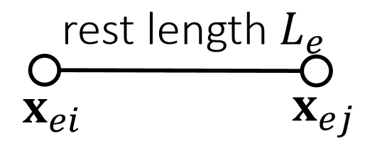
$$ \mathbf{ϕ} _e(\mathbf{x} )=||\mathbf{x} _{ei}− \mathbf{x} _{ej}||−L_e $$
$$ E(\mathbf{x} )={\textstyle \sum_e}\frac{1}{2} k(||\mathbf{x} _{ei} −\mathbf{x} _{ej}||−L_e)^2=\frac{1}{2} \mathbf{\mathbf{ϕ}^T(x)C} ^{−1}\mathbf{ϕ} (\mathbf{x} ) $$
✅ \(E(X)=\sum _ {e} \frac{1}{2}k( \phi _ e(x))^2\)
$$ \mathbf{f} (\mathbf{x} )=−∇E=-\begin{pmatrix} \frac{∂E}{∂\mathbf{ϕ}} & \frac{∂\mathbf{ϕ}}{∂x} \end{pmatrix}^\mathbf{T} =−\mathbf{J^TC} ^{−1}\mathbf{ϕ} =\mathbf{J^Tλ} $$
Let \(N\) be the number of vertices and E be the number of constraints,
| 约束 | $$ \phi (\mathbf{x} )\in \mathbf{R} ^E $$ | ✅ \( \phi_e = \begin{bmatrix} \phi _ 0\\ \phi _ 1 \\ \vdots \\ \phi _ E \end{bmatrix}\) |
| Compliant matrix | $$ \mathbf{C} =\begin{bmatrix} 1/k & \Box & \Box\\ \Box & 1/k & \Box \\ \Box & \Box &\ddots \end{bmatrix}\in \mathbf{R} ^{E×E} $$ | ✅ C称为软度矩阵、 stiffness:挺度,compliant:软度 |
| Jacobian | \(\mathbf{J} =\frac{∂\phi}{∂\mathbf{x} } \in \mathbf{R} ^{E×3N}\) | |
| Dual variables (Lagrangian multipliers) | \(\mathbf{λ} =−\mathbf{C} ^{−1}\phi \in \mathbf{R} ^E\) | ✅ \(\lambda \) 是人为引入的变量,称为拉格朗日算子。 |
✅ \(E\) 和 \(f\) 变成了关于两个变量\((x、\lambda )\)的函数。
✅ 把能量写成约束的形式
$$ E(x)=\frac{1}{2}\phi ^T (x)C^{-1}\lambda \\ f(x)=J^T \lambda
$$ 根据\(E(x)\)和\(f(x)\)做隐式积分
转化为隐式积分问题
P31
By implicit integration, we get:
$$ \mathbf{Mv} ^{\mathrm{new} }−∆t\mathbf{J^Tλ} ^{\mathrm{new} }=\mathbf{Mv} $$
✅ 动量守衡公式:\(Mv'- Mv = Ft = \)冲量
✅ 此处新 \(\lambda^{\mathrm{new}} \)来计算 F. 说明是 Implicit
Meanwhile, $$ \mathbf{Cλ} ^{\mathrm{new} }=−\mathbf{ϕ} ^{\mathrm{new} }≈−\mathbf{ϕ} −\mathbf{J} (\mathbf{x} ^{\mathrm{new} }−\mathbf{x} )≈−\mathbf{ϕ} −∆t\mathbf{Jv} ^{\mathrm{new} } $$
✅ 对\(-\phi ^{\mathrm{new}}\) 的泰勒展开
✅\(J\)是上页中的Jacobian.
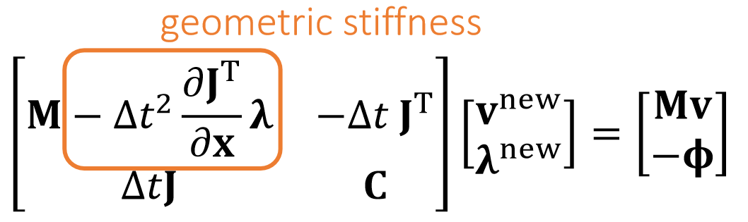
$$ \begin{bmatrix} \mathbf{M} & −∆t\mathbf{J^T} \\ ∆t\mathbf{J} & \mathbf{C} \end{bmatrix}\begin{bmatrix} \mathbf{v} ^{\mathrm{new} } \\ \mathbf{λ} ^{\mathrm{new} } \end{bmatrix}\begin{bmatrix} \mathbf{Mv} \\ -\mathbf{ϕ} \end{bmatrix} $$
✅ 最后的矩阵公式由上面两个公式整理合并得到。
✅ \(x ^{\mathrm{new}}-x =\bigtriangleup t\cdot v \)
解隐式积分
P32
Now we have a system with two sets of variables: the primal variable \(\mathbf {x}\) (or \(\mathbf {v=x}\) ̇) and the dual variable \(\mathbf {λ}\).
✅ 之前的隐式积分只有一个变量,此处的隐式积分有两个变量。需要同时解出两个变量。
- Method 1: We can solve the two variables by a direct solver together, in a primal-dual fashion:
$$ \begin{bmatrix} \mathbf{M} & −∆t\mathbf{J^T} \\ ∆t\mathbf{J} & \mathbf{C} \end{bmatrix}\begin{bmatrix} \mathbf{v} ^{\mathrm{new} } \\ \mathbf{λ} ^{\mathrm{new} } \end{bmatrix} = \begin{bmatrix} \mathbf{Mv} \\ -\mathbf{ϕ} \end{bmatrix} $$
✅ 注意:Method 1 中的矩阵有可能不正定、因此很多数学方法用不了。
- Method 2: We can reduce the system by Schur complement and solve \(\mathbf {λ}^{\mathrm{new} }\) first.
✅ Method 2 的消元过程不容易构造、尤其是当矩阵比较复杂时。
$$ (∆t^2\mathbf{JM} ^{−1}\mathbf{J} ^\mathbf{T} +\mathbf{C} )\mathbf{λ} ^{\mathrm{new} } =−\mathbf{ϕ} −∆t\mathbf{Jv} $$
$$ \mathbf{v} ^{\mathrm{new}}\longleftarrow \mathbf{v} +−∆t\mathbf{M} ^{−1}\mathbf{J^Tλ} ^{\mathrm{new}} $$
✅ 用哪种方法取决于应用场景
优点
Infinite stiffness? \(\mathbf{C \longrightarrow 0}\).
✅ 此方法将软硬度量解耦出来,并用矩阵C来表示,使得可以方便控制软硬度,例如让\(c=0\) 来表示 infinite stiffness.
应用
Articulated Rigid Bodies (ragdoll animation)
P34
Stable Constrained Dynamics
✅ 没有展开讲,见after reading中的论文
From a mass-spring system, we know spring Hessian (tangent stiffness) is:
$$
\mathbf{H} (\mathbf{x} )=∑_{e=(i,j)}\begin{bmatrix}
\Box & \Box & \Box & \Box \\
\Box & \mathbf{H} _e & -\mathbf{H} _e & \Box \\
\Box & -\mathbf{H} _e &\mathbf{H} _e & \Box \\
\Box & \Box & \Box & \Box
\end{bmatrix}
$$
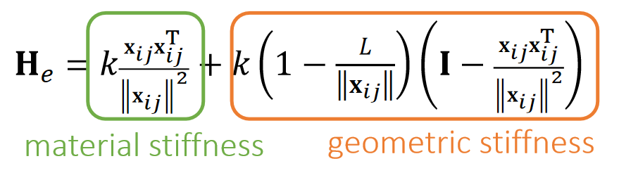
According to constrained dynamics:\(\mathbf{f} (\mathbf{x} )=\mathbf{J^Tλ}\) and \(\mathbf{λ} =−\mathbf{C} ^{−1}\mathbf{ϕ} \), so:
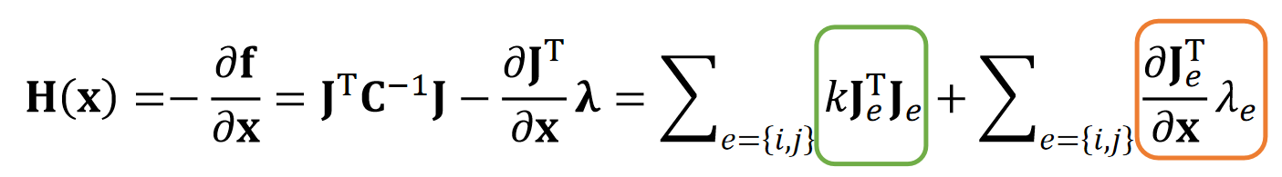
$$ \mathbf{J}_e=\frac{∂\phi _e}{∂\mathbf{x} }=\begin{bmatrix} \frac{\mathbf{x} _{ij}^\mathbf{T} }{||\mathbf{x} _{ij}||} & -\frac{\mathbf{x} _{ij}^\mathbf{T} }{||\mathbf{x} _{ij}||} \end{bmatrix} $$
P35
Stable Constrained Dynamics
According Lecture 5, Page 16, implicit integration is:
$$ (\frac{1}{∆t^2}\mathbf{M+H} (\mathbf{x} ^{[0]}))∆\mathbf{x} = \frac{1}{∆t^2}\mathbf{M} (∆t\mathbf{v} ^{[0]})+\mathbf{f} (\mathbf{x} ^{[0]}) $$
$$ \Downarrow $$
$$ (\mathbf{M} +∆t^2\mathbf{H} (\mathbf{x} ^{[0]}))\mathbf{v} ^{\mathrm{new} }= \mathbf{Mv} ^{[0]}+∆t\mathbf{f} (\mathbf{x} ^{[0]}) $$
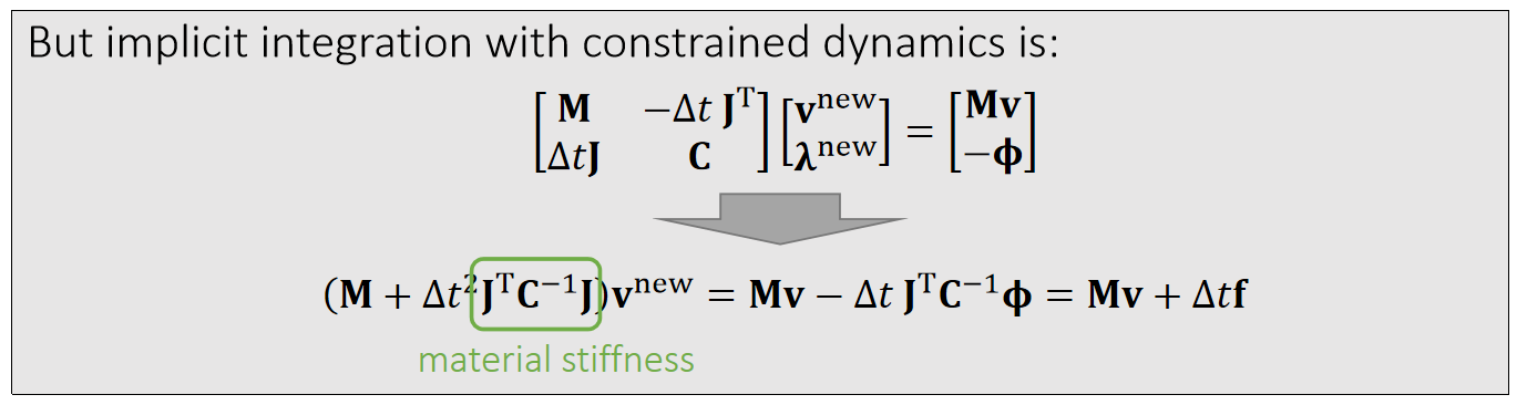
Missing geometric stiffness matrix here…
P36
After-Class Reading (optional)
Tournier et al. 2015. Stable Constrained Dynamics. TOG (SIGGRAPH).
✅ Method 2 Gauss 消元,如果把\(\lambda\)消掉,会得到一个基本上与隐式积分相似的公式,唯一的区别是\(\mathbf{H}\)上略有不同 —— 隐式积分多了一项。如果把用这一项加回去,会使constrain dynamic 变得稳定。
本文出自CaterpillarStudyGroup,转载请注明出处。
https://caterpillarstudygroup.github.io/GAMES103_mdbook/