Introduction
在线阅读地址:https://caterpillarstudygroup.github.io/LiuYuBo_ML_pages/
《python3入门机器学习 经典算法与应用》学习笔记
视频资源链接:https://coding.imooc.com/class/169.html
这套视频课系列原作者刘宇波。课程发布于慕课网。
课程对常见机器学习算法做了基础的介绍。既有原理也有编程实践。还有一些对算法的思考。
在讲原理有少量的数学推导,数学基础不好也能看懂。
简单的算法配有python3实现,复杂算法使用slearn观察算法效果,对算法有直观印象。
适用于机器学习入门,也可用于熟悉python、numpy和sklearn。
这个系列课程不错,墙裂推荐
KNN - K近邻算法 - K-Nearest Neighbors
KNN算法是非常适合入门机器学习的算法,因为
- 思想极度简单
- 应用数学知识少
- 效果好
- 可以解释机器学习算法使用过程中的很多细节问题
- 更完整地刻画机器学习应用的流程
2019-10-19
KNN - K近邻算法 - K-Nearest Neighbors
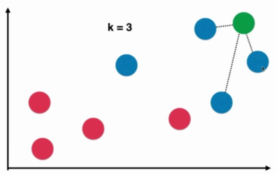
本质:如果两个样本足够相似,它们有更高的概率属于同一个类别
代码实现KNN算法
假设原始训练数据如下:
raw_data_X = [[3.39, 2.33],
              [3.11, 1.78],
              [1.34, 3.36],
              [3.58, 4.67],
              [2.28, 2.86],
              [7.42, 4.69],
              [5.74, 3.53],
              [9.17, 2.51],
              [7.79, 3.42],
              [7.93, 0.79]
             ]
raw_data_y = [0, 0, 0, 0, 0, 1, 1, 1, 1, 1]
待求数据如下:
x = np.array([8.09, 3.36])
数据准备
import numpy as np
import matplotlib.pyplot as plt

X_train = np.array(raw_data_X)
y_train = np.array(raw_data_y)

plt.scatter(X_train[y_train==0, 0], X_train[y_train==0, 1], color = 'g')
plt.scatter(X_train[y_train==1, 0], X_train[y_train==1, 1], color = 'r')
plt.scatter(x[0], x[1], color = 'b')
plt.show()
效果:

KNN过程
欧拉距离
假设有a, b两个点,平面中两个点之间的欧拉距离为:
$$ \sqrt {(x^{(a)}-x^{(b)})^2+(y^{(a)}-y^{(b)})^2} $$
立体中两个点的欧拉距离为:
$$ \sqrt {(x^{(a)}-x^{(b)})^2+(y^{(a)}-y^{(b)})^2+(z^{(a)}-z^{(b)})^2} $$
任意维度中两个点的欧拉距离为:
$$ \sqrt {(X^{(a)}_1-X^{(b)}_1)^2+ (X^{(a)}_2-X^{(b)}_2)^2+...+(X^{(a)}_n-X^{(b)}_n)^2} $$
或
$$ \sqrt {\sum^n_{i=1} (X^{(a)}_i-X^{(b)}_i)^2} $$
其中上标a, b代码第a, b个数据。下标1, 2代码数据的第1, 2个特征
代码如下:
distances = [np.sum((x_train - x) ** 2) for x_train in X_train]
nearest = np.argsort(distances)
topK_y = [y_train[i] for i in nearest[:k]]
from collections import Counter
votes = Counter(topK_y)
predict_y = votes.most_common(1)[0][0]
运行结果:predict_y = 1
代码实现KNN算法
import numpy as np
from math import sqrt
from collections import Counter

def kNN_classify(k, X_train, y_train, x):
    assert 1 <= k <= X_train.shape[0], "k must be valid"
    assert X_train.shape[0] == y_train.shape[0], "the size of X_train must equal to the size of y_train"
    assert X_train.shape[1] == x.shape[0], "the feature number of x must be equal to X_train"

    distances = [sqrt(np.sum((x_train-x)**2)) for x_train in X_train]
    nearst = np.argsort(distances)

    topK_y = [y_train[i] for i in nearst[:k]]
    votes = Counter(topK_y)

    return votes.most_common(1)[0][0]
准备数据
import numpy as np
raw_data_X = [[3.39, 2.33],
              [3.11, 1.78],
              [1.34, 3.36],
              [3.58, 4.67],
              [2.28, 2.86],
              [7.42, 4.69],
              [5.74, 3.53],
              [9.17, 2.51],
              [7.79, 3.42],
              [7.93, 0.79]
             ]
raw_data_y = [0, 0, 0, 0, 0, 1, 1, 1, 1, 1]

X_train = raw_data_X
y_train = raw_data_y

x = np.array([8.09, 3.36])
调用算法
predict_y = kNN_classify(6, X_train, y_train, x)
运行结果:predict_y = 1
什么是机器学习
KNN是一个不需要训练的算法
KNN没有模型,或者说训练数据就是它的模型
使用scikit-learn中的kNN
错误写法
from sklearn.neighbors import KNeighborsClassifier

kNN_classifier.fit(X_train, y_train)
kNN_classifier.predict(x)
这样写会报错:
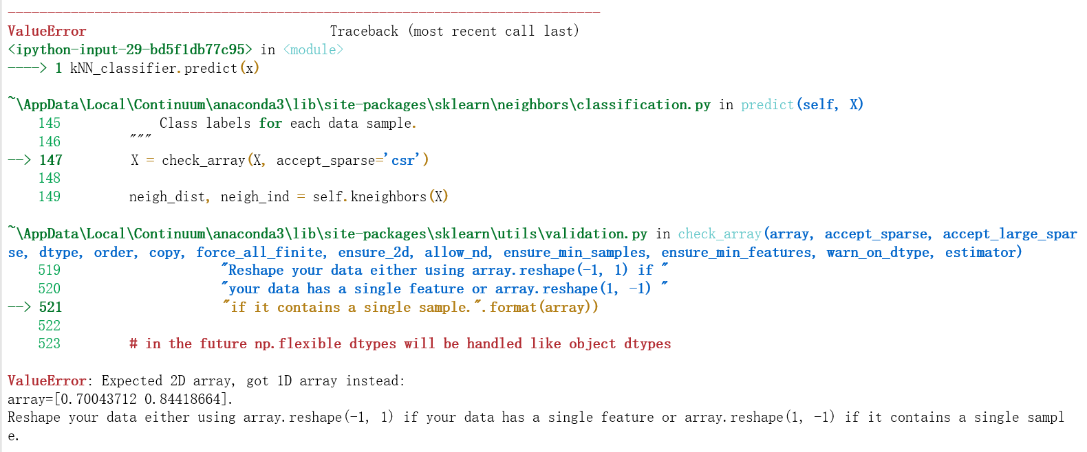
原因是,predict为了兼容多组测试数据的场景,要求参数是个矩阵
正确写法
from sklearn.neighbors import KNeighborsClassifier

kNN_classifier.fit(X_train, y_train)
X_predict = x.reshape(1, -1)
y_predict = kNN_classifier.predict(X_predict)
运行结果:predict_y[0] = 1
重新整理我们的kNN的代码
封装成sklearn风格的类
import numpy as np
from math import sqrt
from collections import Counter

class kNNClassifier:

    def __init__(self, k):
        """初始化kNN分类器"""
        assert k >= 1, "K must be valid!"
        self.k = k
        self._X_train = None
        self._y_train = None

    def fit(self, X_train, y_train):
        """根据训练数据集X_train和y_train训练kNN分类器"""
        assert X_train.shape[0] == y_train.shape[0], "the size of X_train must equal to the size of y_train"
        assert self.k <= X_train.shape[0], "the size of X_train must be at least k"

        self._X_train = X_train
        self._y_train = y_train
        return self

    def predict(self, X_predict):
        """给定待预测数据集X_predict, 返回表示X_predict的结果向量"""
        assert self._X_train is not None and self._X_train is not None, "must fit before predict"
        assert self._X_train.shape[1] == X_predict.shape[1], "the feature number of X_predict must be equal to X_train"

        y_predict = [self._predict(x) for x in X_predict]
        return np.array(y_predict)

    def _predict(self, x):
        """给定单个待测数据x,返回x的预测结果"""
        assert self._X_train.shape[1] == x.shape[0], "the feature number of x must be equal to X_train"

        distances = [sqrt(np.sum((x_train-x)**2)) for x_train in self._X_train]
        nearst = np.argsort(distances)

        topK_y = [self._y_train[i] for i in nearst[:self.k]]
        votes = Counter(topK_y)

        return votes.most_common(1)[0][0]

    def __repr__(self):
        return "KNN(k=%d)" % self.k
使用kNNClassifier
knn_clf = kNNClassifier(k=6)
knn_clf.fit(X_train, y_train)
y_predict = knn_clf.predict(X_predict)
运行结果:predict_y[0] = 1
判断机器学习算法的性能

改进:训练和测试数据集的分离,train test split

但这种方式也有它的问题,后面其它小节会讲到
准备iris数据
import numpy as np
import matplotlib.pyplot as plt
from sklearn import datasets

iris = datasets.load_iris()
X = iris.data
y = iris.target
X.shape为(150, 4),y.shape为(150,)
train_test_split
注意1:本例中训练数据集的为如下:

因此按顺序取前多少个样本不会有很好的效果,要先对数据乱序化
注意2:本例中X和y是分离的,但它们不能分别乱序化。乱序化的同时要保证样本和标签是对应的。
在Notebook实现
shuffle_indexes = np.random.permutation(len(X))
test_ratio = 0.2
test_size = int(len(x) * test_ratio)
test_indexes = shuffle_indexes[:test_size]
train_indexes = shuffle_indexes[test_size:]

X_train = X[train_indexes]
y_train = y[train_indexes]
X_test = X[test_indexes]
y_test = y[test_indexes]
将train_test_split封装成函数
import numpy as np

def train_test_split(X, y, test_ratio=0.2, seed=None):
    """将X和y按照test_ratio分割成X_train,X_test,y_train,y_test"""

    assert X.shape[0] == y.shape[0], "the size of X must be equal to the size of y"
    assert 0.0 <= test_ratio <= 1.0, "test_ration must be valid"

    if seed:
        np.random.seed(seed)

    shuffle_indexes = np.random.permutation(len(X))

    test_size = int(len(x) * test_ratio)
    test_indexes = shuffle_indexes[:test_size]
    train_indexes = shuffle_indexes[test_size:]

    X_train = X[train_indexes]
    y_train = y[train_indexes]

    X_test = X[test_indexes]
    y_test = y[test_indexes]

    return X_train, X_test, y_train, y_test
KNN结合train_test_split计算分类准确度
X_train, X_test, y_train, y_test = train_test_split(X, y)
my_Knn_clf = kNNClassifier(k = 3)    # kNNClassifier在上一节实现
my_Knn_clf.fit(X_train, y_train)
y_predict = my_Knn_clf.predict(X_test)
accuracy = sum(y_predict == y_test) / len(y_test)
sklearn中的train_test_split
from sklearn.model_selection import train_test_split
X_train, X_test, y_train, y_test = train_test_split(X, y, test_size=0.2, random_state=666)
在4-3中使用了分类准确度accuracy来评判KNN算法的性能。
使用accuracy来评价KNN算法对手写数据集的分类效果
加载手写数据集
from sklearn import datasets
digits = datasets.load_digits()
digits的内容如下:
输入:digits.keys()
输出:dict_keys(['data', 'target', 'target_names', 'images', 'DESCR'])
输入:print(digits.DESCR)
输出:digits的官方说明
输入:digits.data.shape()
输出:(1797, 64)
输入:digits.target.shape()
输出:(1797,)
输入:digits.target_names
输出:array([0, 1, 2, 3, 4, 5, 6, 7, 8, 9])
输入:
some_digit = X[666]

some_digit_image = some_digit.reshape(8, 8)
plt.imshow(some_digit_image, cmap = matplotlib.cm.binary)
plt.show()
输出:第666个样本的图像

train_test_split + KNN + accuracy
import numpy as np
import matplotlib
import matplotlib.pyplot as plt
from sklearn import datasets

digits = datasets.load_digits()
X = digits.data
y = digits.target

X_train, X_test, y_train, y_test = train_test_split(X, y, test_ratio=0.2)
my_knn_clf = KNNClassifier(k=3)
my_knn_clf.fit(X_train, y_train)
y_predict = my_knn_clf.predict(X_test)
accuracy = sum(y_predict == y_test) / len(y_test)
scikit-learn中的accuracy_score
from sklearn.model_selection import train_test_split
X_train, X_test, y_train, y_test = train_test_split(X, y, test_size=0.2, random_state=666)

from sklearn.neighbors import KNeighborsClassifier
knn_clf = KNeighborsClassifier(n_neighbors=3)

knn_clf.fit(X_train, y_train)
y_predict = knn_clf.predict(X_test)

from sklearn.metrics import accuracy_score
accuracy = accuracy_score(y_test, y_predict)
超参数和模型参数
超参数是指运行机器学习算法之前要指定的参数
KNN算法中的K就是一个超参数
模型参数:算法过程中学习的参数
KNN算法没有模型参数
调参是指调超参数
如何寻找好的超参数
- 领域知识
- 经验数值
- 实验搜索
寻找最好的K
best_score = 0.0
best_k = -1
for k in range(1, 11):
    knn_clf = KNeighborsClassifier(n_neighbors=k)
    knn_clf.fit(X_train, y_train)
    score = knn_clf.score(X_test, y_test)
    if score > best_score:
        best_k = k
        best_score = score

print("best_k = ", best_k)
print("best_score = ", best_score)
输出:
best_k = 4
best_score = 0.9916666666666667
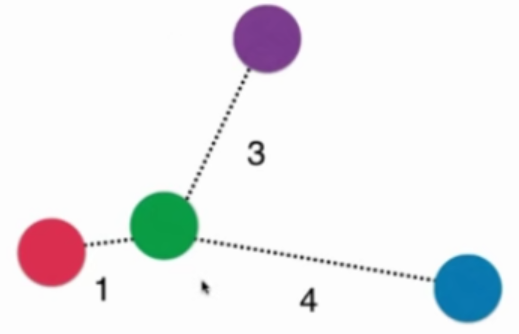
KNN的超参数weights
-
普通的KNN算法:蓝色获胜
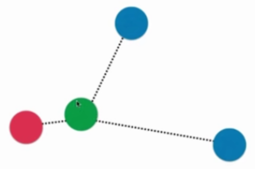
-
考虑距离的KNN算法:红色:1, 蓝色:1/3 + 1/4 = 7/12,蓝色获胜
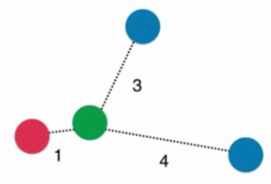
考虑距离的另一个优点:解决平票的情况
best_method = ""
best_score = 0.0
best_k = -1
for method in ["uniform", "distance"]:
    for k in range(1, 11):
        knn_clf = KNeighborsClassifier(n_neighbors=k, weights=method)
        knn_clf.fit(X_train, y_train)
        score = knn_clf.score(X_test, y_test)
        if score > best_score:
            best_k = k
            best_score = score
            best_method = method

print("best_k = ", best_k)
print("best_score = ", best_score)
print("best_method = ", best_method)
输出结果:
best_k = 4
best_score = 0.9916666666666667
best_method = uniform
KNN的超参数p
关于距离的更多定义
- 欧拉距离
$$ \sqrt {\sum^n_{i=1} (X^{(a)}_i-X^{(b)}_i)^2} $$
- 曼哈顿距离
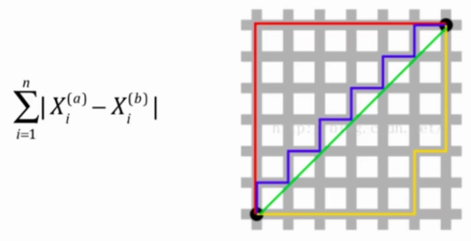
- 欧拉距离与曼哈顿距离的数学形式一致性
$$ (\sum^n_{i=1} |X^{(a)}_i-X^{(b)}_i|^2)^\frac{1}{2} $$
$$ (\sum^n_{i=1} |X^{(a)}_i-X^{(b)}_i|)^\frac{1}{1} $$
- 明可夫斯基距离 Minkowski distance
$$ (\sum^n_{i=1} |X^{(a)}_i-X^{(b)}_i|^p)^\frac{1}{p} $$
把欧拉距离和曼哈顿距离进一步抽象,得到以下公式

p = 1: 曼哈顿距离
p = 2: 欧拉距离
p > 2: 其他数学意义
%%time

best_p = -1
best_score = 0.0
best_k = -1

for k in range(1, 11):
    for p in range(1, 6):
        knn_clf = KNeighborsClassifier(n_neighbors=k, weights="distance", p = p)
        knn_clf.fit(X_train, y_train)
        score = knn_clf.score(X_test, y_test)
        if score > best_score:
            best_k = k
            best_score = score
            best_p = p

print("best_k = ", best_k)
print("best_score = ", best_score)
print("best_p = ", best_p)
输出结果:
best_k = 3
best_score = 0.9888888888888889
best_p = 2
Wall time: 37 s
Grid Search
准备数据
from sklearn import datasets

digits = datasets.load_digits()
X = digits.data
y = digits.target

from sklearn.model_selection import train_test_split
X_train, X_test, y_train, y_test = train_test_split(X, y, test_size=0.2, random_state=666)
使用网格搜索
from sklearn.neighbors import KNeighborsClassifier
from sklearn.model_selection import GridSearchCV

param_grid = [
    {
        'weights':['uniform'],
        'n_neighbors': [i for i in range(1, 11)]
    },
    {
        'weights':['distance'],
        'n_neighbors': [i for i in range(1, 11)],
        'p': [i for i in range(1, 6)]
    }
]

knn_clf = KNeighborsClassifier()
grid_search = GridSearchCV(knn_clf, param_grid)

%%time
grid_search.fit(X_train, y_train)
输出结果:

察看运行结果
输入:grid_search.best_score_
输出:0.9853862212943633
输入:grid_search.best_params_
输出:{'n_neighbors': 3, 'p': 3, 'weights': 'distance'}
注意1:这里的搜索结果与4-5中自己编写的网格搜索得到的结果不同,是因为评价方法不同,不用care
注意2:以_结尾的参考表示为计算得到的参数,而不是用户输入的参数
使用运行结果建立新的模型
knn_clf = grid_search.best_estimator_
knn_clf.score(X_test, y_test)
输出结果: 0.9833333333333333
其它GridSearchCV参数
- njobs:使用多核计算
- verbose:中间过程的打印级别
更多的距离定义


样本间的距离被发现时间所主导
如果把发现时间改成以年为单位,样本间的距离又会被肿瘤大小所主导
如果不对样本进行预处理,样本间的距离可能会被部分特征主导
解决方案:将所有的数据映射到同一个尺度,即归一化
数据归一化 (feature scaling)
最值归一化 normalization
把所有数据映射到0-1之间
$$ x_{scale} = \frac {x - x_{min}}{x_{max} - x_{min}} $$
适用于分布有明显边界的情况,但是受outlier也就是极值(极端数据)影响较大会不准确
均值方差归一化 standardization
把所有数据归一到均值为0方差为1的分布中
$$ x_{scale} = \frac {x-x_{mean}}{S} $$
适用于数据分布没有明显的边界,有可能存在极端的数据值,其中S是标准差。由于均值方差归一化对于符合最值归一化的数据集有着同样好的归一化处理结果,所以一般推荐使用均值方差归一化方法。
代码实现归一化
最值归一化
对向量所有元素归一化
生成随机数据
x = np.random.randint(0, 100, size = 100)

归一化后
(x - np.min(x)) / (np.max(x) - np.min(x))

对矩阵元素归一化
X = np.random.randint(0, 100, (50, 2))
X = np.array(X, dtype = float)
X[:, 0] = (X[:,0] - np.min(X[:,0])) / (np.max(X[:,0])-np.min(X[:,0]))
X[:, 1] = (X[:,1] - np.min(X[:,1])) / (np.max(X[:,1])-np.min(X[:,1]))
均值方差归一化 standardization
X2 = np.random.randint(0, 100, (50, 2))
X2 = np.array(X2, dtype = float)

X2[:,0] = (X2[:,0] - np.mean(X2[:,0])) / np.std(X2[:,0])
X2[:,1] = (X2[:,1] - np.mean(X2[:,1])) / np.std(X2[:,1])
输入:np.mean(X2[:,0])
输出:7.771561172376095e-17
输入:np.std(X2[:,0])
输出:1.0
训练数据集和测试数据集不能分别归一化。
测试数据集使用与训练数据集相同的mean和std做归一化
即
(x_test - mean_train) / std_train
scikit-learn中的Scaler的使用流程

使用scikit-learn中的StandardScaler
准备数据
import numpy as np
from sklearn import datasets

iris = datasets.load_iris()
X = iris.data
y = iris.target

from sklearn.model_selection import train_test_split

X_train, X_test, y_train, y_test = train_test_split(iris.data, iris.target, random_state=666)
scikit-learn中的StandardScaler
from sklearn.preprocessing import StandardScaler

standardScaler = StandardScaler()
standardScaler.fit(X_train)

X_train_standard = standardScaler.transform(X_train)
X_test_standard = standardScaler.transform(X_test)
StandardScaler + KNN + accuracy
from sklearn.neighbors import KNeighborsClassifier
knn_clf = KNeighborsClassifier(n_neighbors=3)
knn_clf.fit(X_train_standard, y_train)
knn_clf.score(X_test_standard, y_test)
自己实现StandardScaler并封装成类
import numpy as np

class StandardScaler:

    def __init__(self):
        self.mean_ = None
        self.scale_ = None

    def fit(self, X):
        """根据训练数据集X获取数据的均值和方差"""
        assert X.ndim == 2, "The dimension of X must be 2"

        self.mean_ = np.array([np.mean(X[:,i]) for i in range(X.shape[1])])
        self.scale_ = np.array([np.std(X[:,i]) for i in range(X.shape[1])])

    def transform(self, X):
        """将X根据这个StandardScaler进行均值方差归一化处理"""
        assert X.ndim == 2, "The dimension of X must be 2"
        assert self.mean_ is not None and self.scale_ is not None, "must fit before transform!"

        retX = np.empty(shape = X.shape, type = float)
        for col in range(X.shape[1]):
            retX[:, col] = (X[:,col] - self.mean_[col]) / self.scale_[col]
        return retX
优点:
解决分类问题,天然可以解决多分类问题
思想简单,效果强大
可以解决回归问题:KNeighborsRegressor
缺点:
效率低下,m个特征n个样本,预测一个数据的时间复杂度为O(m * n)
高度数据相关
预测结果不所有可解释性
维数灾难:随着维度的增加,看似相近的两个点距离越来越大,解决方法:降维
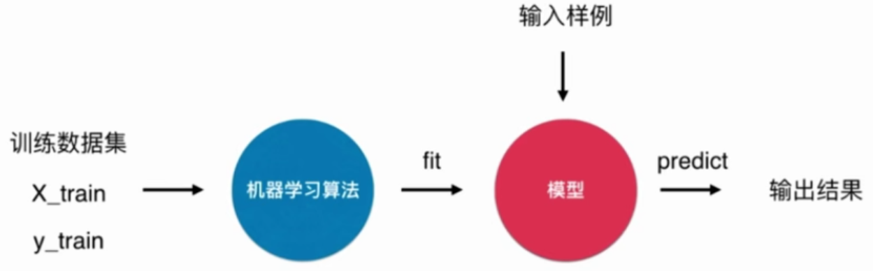
机器学习流程回顾

线性回归算法
解决回归问题
思想简单、实现容易
许多强大的非线性模型的基础
结果具有很好的可解释性
蕴含机器学习中的很多重要思想
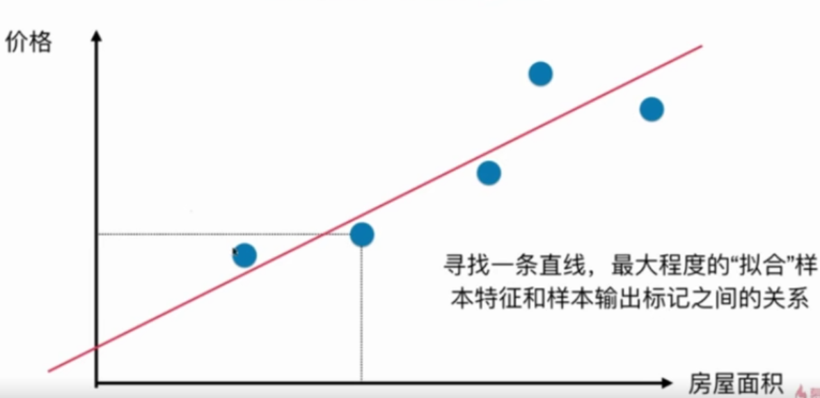
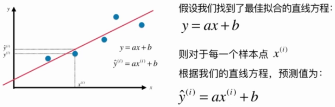
注意1:这里的二维平面图与分类问题的二维平面图不同
在分类问题中,横轴和纵轴都是样本特征,输出标记用颜色表示
在回归问题中,横轴是样本特征,纵轴是输出标记
注意2:
样本特征只有一个,称为简单线性回归
样本特征有多个,称为多元线性回归
简单线性回归
找一条直线,这条直线最大程度地拟合所有的样本特征点
一类机器学习算法的基本思路
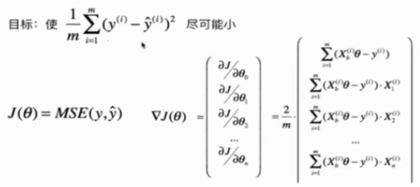
通过分析问题,确定问题的损失函数(loss function)或效用函数(utility function), 有时也称为目标函数
通过最优化损失函数或效用函数,获得机器学习的模型
近乎所有的参数学习算法都是这样的套路, e.g. 线性回归, 多项式回归, 逻辑回归, SVM, 神经网络, etc...本质都是在学习相应的参数来最优化目标函数, 区别在于模型不同从而建立的目标函数不同, 优化的方式也不尽相同.
最优化原理
凸优化
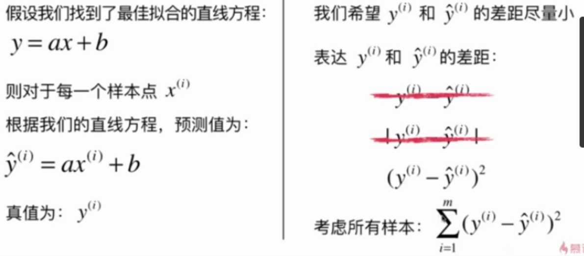
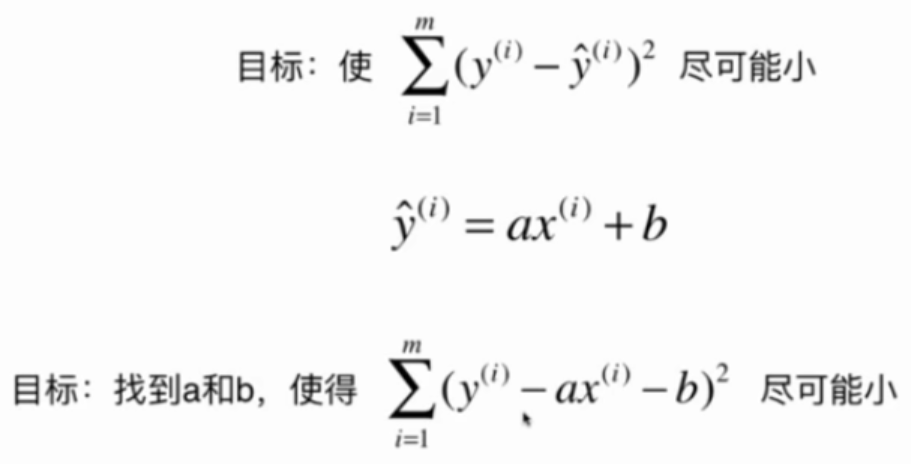
最小化本文中的损失函数
目标:找到$${a}$$和$${b}$$,使用$$\sum^m_{i=1}(y^{(i)}-ax^{(i)}-b)^2$$尽可能小。
这是典型的最小二乘法问题:最小化误差的平方
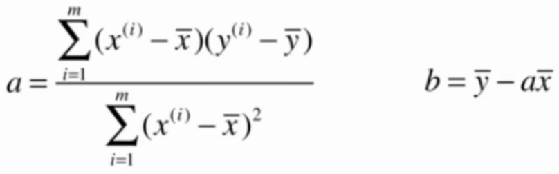
解得:
$$ a = \frac{\sum_{i=1}^m(x^{(i)}-\bar x)(y^{(i)}-\bar y)}{\sum_{i=1}^m(x^{(i)}-\bar x)^2}\quad \quad \quad \quad \quad b = \bar y - a\bar x $$
5-1中的a和b的证明过程
这一节没有做笔记
import numpy as np
import matplotlib.pyplot as plt
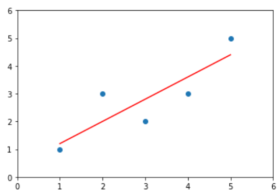
x = np.array([1., 2., 3., 4., 5.])
y = np.array([1., 3., 2.
plt.scatter(x, y)
plt.axis([0, 6, 0, 6])
plt.show()
输出结果:

在Notebook中计算a, b
计算a, b
x_mean = np.mean(x)
y_mean = np.mean(y)

num = 0.0
d = 0.0
for x_i, y_i in zip(x, y):
    num += (x_i - x_mean) * (y_i - y_mean)
    d += (x_i - x_mean) ** 2

a = num / d
b = y_mean - a * x_mean
绘制结果
y_hat = a * x + b

plt.scatter(x, y)
plt.plot(x, y_hat, color='r')
plt.axis([0, 6, 0, 6])
plt.show()
输出结果:
把上过程封装成类
import numpy as np

class SimpleLinearRegression1:
    def __init__(self):
        """初始化Single Linear Regression模型"""
        self.a_ = None
        self.b_ = None

    def fit(self, x_train, y_train):
        """根据训练数据集X_train, y_train训练Single Linear Regression模型"""
        assert x_train.ndim == 1, "Simple Linear Regressor can only solve single feature training data"
        assert len(x_train) == len(y_train), "the size of x_train must be equal to the size of y_train"

        x_mean = np.mean(x_train)
        y_mean = np.mean(y_train)

        num = 0.0
        d = 0.0
        for x_i, y_i in zip(x_train, y_train):
            num += (x_i - x_mean) * (y_i - y_mean)
            d += (x_i - x_mean) ** 2

        self.a_ = num / d
        self.b_ = y_mean - self.a_ * x_mean

    def predict(self, x_predict):
        """给定待测数据集X_predict,返回表示x_predict的结果向量"""
        assert x_predict.ndim == 1, "Simple Linear Regressor can only solve single feature training data"
        assert self.a_ is not None and self.b_ is not None, "must fit before predict"
        return [self._predict(x) for x in x_predict]

    def _predict(self, x_single):
        """给定单个待预测数据s_single,返回x_single的预测结果"""
        return self.a_ * x_single + self.b_

    def __repr__(self):
        return "SimpleLinearRegression1()"
训练模型
reg1 = SimpleLinearRegression1()
reg1.fit(x, y)
绘制结果
y_hat1 = a * x + b

plt.scatter(x, y)
plt.plot(x, y_hat1, color='r')
plt.axis([0, 6, 0, 6])
plt.show()
输出结果:
5-3中计算a, b的实现方法性能较低,使用向量化运算能提高性能
即把以下公式向量化:
向量化的依据:
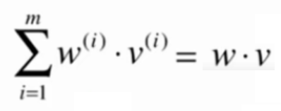
向量化计算a, b
import numpy as np

class SimpleLinearRegression2:
    def __init__(self):
        """初始化Single Linear Regression模型"""
        self.a_ = None
        self.b_ = None

    def fit(self, x_train, y_train):
        """根据训练数据集X_train, y_train训练Single Linear Regression模型"""
        assert x_train.ndim == 1, "Simple Linear Regressor can only solve single feature training data"
        assert len(x_train) == len(y_train), "the size of x_train must be equal to the size of y_train"

        x_mean = np.mean(x_train)
        y_mean = np.mean(y_train)

        num = (x_train - x_mean).dot(y_train - y_mean)
        d = (x_train - x_mean).dot(x_train - x_mean)

        self.a_ = num / d
        self.b_ = y_mean - self.a_ * x_mean

    def predict(self, x_predict):
        """给定待测数据集X_predict,返回表示x_predict的结果向量"""
        assert x_predict.ndim == 1, "Simple Linear Regressor can only solve single feature training data"
        assert self.a_ is not None and self.b_ is not None, "must fit before predict"
        return [self._predict(x) for x in x_predict]

    def _predict(self, x_single):
        """给定单个待预测数据s_single,返回x_single的预测结果"""
        return self.a_ * x_single + self.b_

    def __repr__(self):
        return "SimpleLinearRegression2()"
绘制结果
import numpy as np
import matplotlib.pyplot as plt

x = np.array([1., 2., 3., 4., 5.])
y = np.array([1., 3., 2., 3., 5.])

reg2 = SimpleLinearRegression2()
reg2.fit(x, y)

y_hat2 = reg2.predict(x)

plt.scatter(x, y)
plt.plot(x, y_hat2, color='r')
plt.axis([0, 6, 0, 6])
plt.show()
输出结果:
向量化实现的性能测试
m = 1000000
big_x = np.random.random(size = m)
big_y = big_x * 3.0 + 2.0 + np.random.normal(size = m)

%timeit reg1.fit(big_x, big_y)    # reg1见5-4
%timeit reg2.fit(big_x, big_y)
输出结果:
1.15 s ± 12.7 ms per loop (mean ± std. dev. of 7 runs, 1 loop each)
25.2 ms ± 2.08 ms per loop (mean ± std. dev. of 7 runs, 10 loops each)
可见向量化计算能大幅度地提高性能,因此能用向量化计算的地方尽量用向量化计算
分类问题使用accuracy来评价分类结果。
回归问题怎样评价预测结果?
MSE RMSE MAE
均方误差 MSE Mean Squared Error
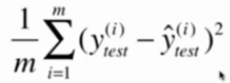
问题:量纲
均方根误差 RMSE Root Mean Squared Error
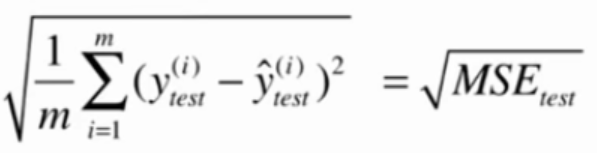 与MSE本质上是一样的
放大了最大的错误
平均绝对误差 MAE Mean Absolute Error

训练过程中,没有把这个函数定义成目标函数,是因为它不是处处可导。
但它仍可以用于评价算法
评价一个算法所使用的标准可以和训练时所用的标准不同
编程实现三种
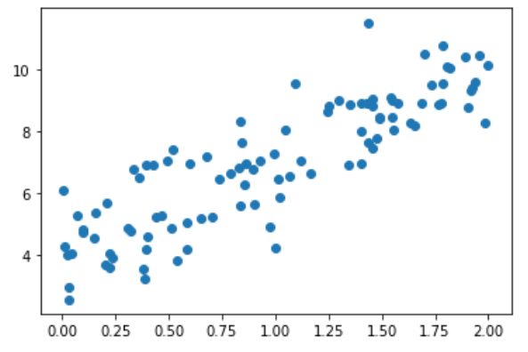
波士顿房产数据
import numpy as np
import matplotlib.pyplot as plt
from sklearn import datasets

boston = datasets.load_boston()
x = boston.data[:, 5] # 5代码房间数,保使用房间数量这个特征
y = boston.target

plt.scatter(x, y)
plt.show()
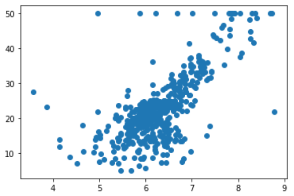
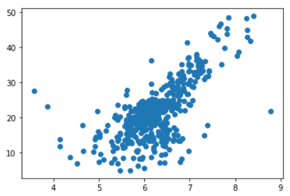
图中最上面有一排点比较奇怪,把它们去掉
x = x[y < 50.0]
y = y[y < 50.0]
plt.scatter(x, y)
plt.show()
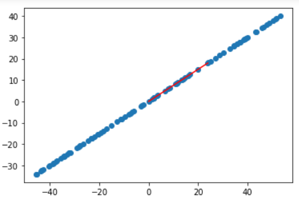
训练模型,预测结果
from sklearn.model_selection import train_test_split
x_train, x_test, y_train, y_test = train_test_split(x, y, test_size=0.2, random_state=666)

reg = SimpleLinearRegression()  #见5-4
reg.fit(x_train, y_train)

plt.scatter(x_train, y_train)
plt.plot(x_train, reg.predict(x_train), color='r')
plt.show()

评价预测效果
y_predict = reg.predict(x_test)

mse_test = np.sum((y_predict - y_test) ** 2) / len(y_test)

from math import sqrt
rmse_test = sqrt(mse_test)

mae_test = np.sum(np.absolute(y_predict-y_test)) / len(y_test)
使用scikit-learn中的MSE和MAE
from sklearn.metrics import mean_squared_error
from sklearn.metrics import mean_absolute_error

mean_squared_error(y_test, y_predict)
mean_absolute_error(y_test, y_predict)
scikit-learn中没有提供RMSE
RMSE vs MAE
量纲相同
RMSE比MSE大
RMSE有放大y_hat与y较大差距的那个值的趋式
让RMSE更小的意义更大
分类问题使用accuracy来评价分类结果。
1最好,0最差。
即使分类的问题不同,也能很容易的比较它们之间的优劣。
但RMSE和MAE无些特性。
解决方法:R Squared
R Squared
$$ R^2 = 1 - \frac {SS_{residual}}{SS_{total}} = 1 - \frac{\sum_i(\hat y^{(i)}- y^{(i)})^2}{\sum_i(\bar y- y^{(i)})^2} $$
说明:
$$SS_{residual}$$: 使用模型预测产生的错误
$$SS_{total}$$: 把所有样本都预测为$$\bar y$$产生的错误
$$\bar y$$:y的平均值
$$\hat y^{(i)}$$:第i个样本的模型预测值
R Squared代表我们的模型拟合住的数据
R Squared的性质:
- R Squared <= 1
- R Squared越大越好。当我们的预测模型不犯任何错误时,R Squared达到最大值1
- 当我们的模型等于基准模型时,R Squared = 0
- 如果R Squared < 0,说明我们的模型还不如基准模型。此时很有可能数据不存在任何线性关系。
R Squared也可以写成这种形式:
 其中Var(y)代表方差
编程实现R Squared
继续使用5-4中的数据和训练结果
1 - mean_squared_error(y_test, y_predict)/np.var(y_test)
或
from sklearn.metrics import r2_score
r2_score(y_test, y_predict)
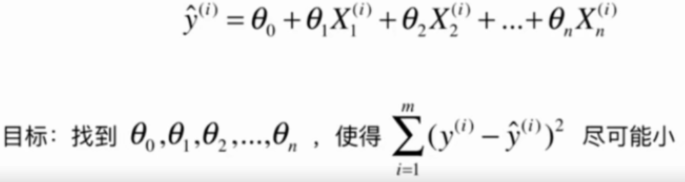
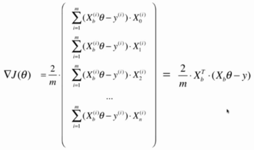
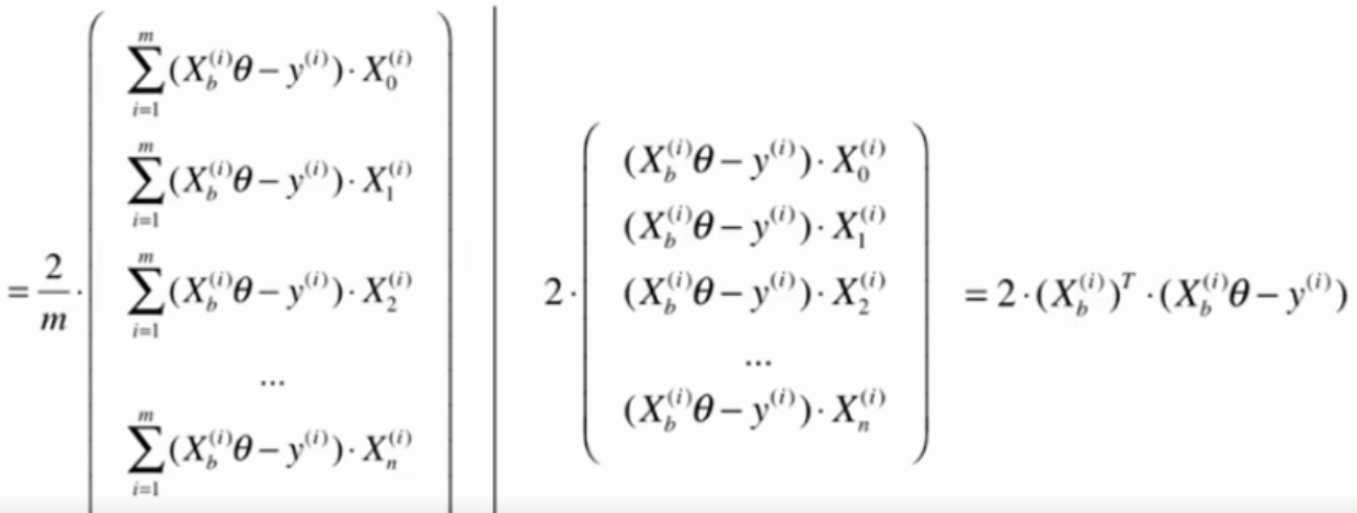
化简结果:
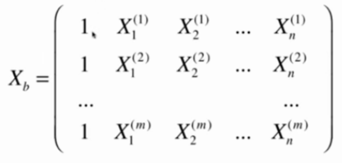
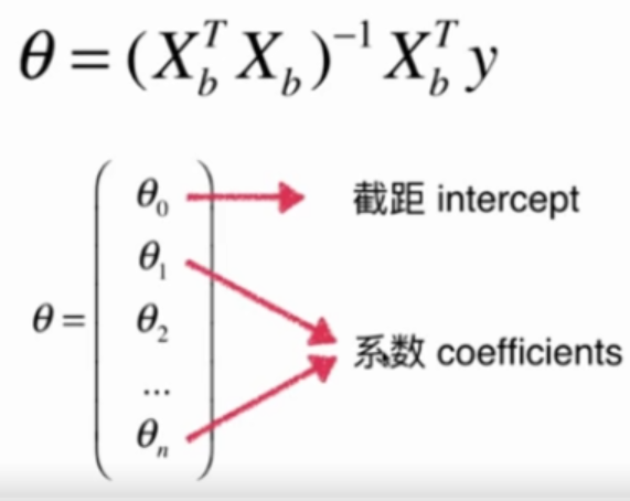
构造矩阵Xb
 要使目标函数最小,必须满足

直接使用这个公式求解,
缺点:时间复杂度太高,O(n^3)
优点:不需要对数据进行规一化
Linear Regression
import numpy as np
from sklearn.metrics import r2_score

class LinearRegression:

    def __init__(self):
        """初始化Linear Regression模型"""
        self.coef_ = None
        self.interception_ = None
        self._theta = None

    def fit_normal(self, X_train, y_train):
        """根据训练数据集X_train, y_train训练Linear Regression模型"""
        assert X_train.shape[0] == y_train.shape[0], "the size of X_train must be equal to the size of y_train"

        X_b = np.hstack([np.ones((len(X_train), 1)), X_train])
        self._theta = np.linalg.inv(X_b.T.dot(X_b)).dot(X_b.T).dot(y_train)

        self.interception_ = self._theta[0]
        self.coef_ = self._theta[1:]

        return self

    def predict(self, X_predict):
        """给定待预测数据集X_predict,返回表示X_predict的结果向量"""
        assert self.interception_ is not None and self.coef_ is not None, "must fit before predict"
        assert X_predict.shape[1] == len(self.coef_), "the feature number of X_predict must equal to X_train"

        X_b = np.hstack([np.ones((len(X_predict), 1)), X_predict])
        return X_b.dot(self._theta)

    def score(self, X_test, y_test):
        """根据测试数据集X_test, y_test确定当前模型的准确度"""

        y_predict = self.predict(X_test)
        return r2_score(y_test, y_predict)

    def __repr__(self):
        return "LinearRegression()"
boston data
import matplotlib.pyplot as plt
from sklearn import datasets

boston = datasets.load_boston()
x = boston.data
y = boston.target
x = x[y < 50.0]
y = y[y < 50.0]
训练模型与预测结果
from sklearn.model_selection import train_test_split
X_train, X_test, y_train, y_test = train_test_split(x, y, test_size=0.2, random_state=666)

reg = LinearRegression()
reg.fit_normal(X_train, y_train)
reg.score(X_test, y_test)
输出结果:
0.8129794056212832
使用多个特征训练的模型得分要高于使用单个特征训练的模型
import matplotlib.pyplot as plt
from sklearn import datasets

boston = datasets.load_boston()
x = boston.data
y = boston.target
x = x[y < 50.0]
y = y[y < 50.0]
Linear Regression
from sklearn.model_selection import train_test_split
X_train, X_test, y_train, y_test = train_test_split(x, y, test_size=0.2, random_state=666)

from sklearn.linear_model import LinearRegression

lin_reg = LinearRegression()
lin_reg.fit(X_train, y_train)
lin_reg.score(X_test, y_test)
KNN Regressor
默认算法
from sklearn.neighbors import KNeighborsRegressor

knn_reg = KNeighborsRegressor()
knn_reg.fit(X_train, y_train)
knn_reg.score(X_test, y_test)
网络搜索
from sklearn.neighbors import KNeighborsRegressor
from sklearn.model_selection import GridSearchCV

param_grid = [
    {
        'weights':['uniform'],
        'n_neighbors': [i for i in range(1, 11)]
    },
    {
        'weights':['distance'],
        'n_neighbors': [i for i in range(1, 11)],
        'p': [i for i in range(1, 6)]
    }
]

knn_reg = KNeighborsRegressor()
grid_search = GridSearchCV(knn_reg, param_grid, n_jobs=-1, verbose=1)
grid_search.fit(X_train, y_train)
输入:grid_search.best_params_
输出:{'n_neighbors': 5, 'p': 1, 'weights': 'distance'}
输入:grid_search.best_score_
输出:0.6340477954176972
输入:grid_search.best_estimator_.score(X_test, y_test)
输出:0.7044357727037996
import matplotlib.pyplot as plt
from sklearn import datasets

boston = datasets.load_boston()
X = boston.data
y = boston.target
X = X[y < 50.0]
y = y[y < 50.0]

from sklearn.linear_model import LinearRegression
lin_reg = LinearRegression()
lin_reg.fit(X, y)

lin_reg.coef_
输出结果:
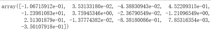
怎么解释这些数字?
- 系数的正负代表这个特征与房价是正相关还是负相关
- 系数的绝对值大小代码这个特征对房价的影响程度
输入:boston.feature_names[np.argsort(lin_reg.coef_)]
输出:
array(['NOX', 'DIS', 'PTRATIO', 'LSTAT', 'CRIM', 'INDUS', 'AGE', 'TAX',
       'B', 'ZN', 'RAD', 'CHAS', 'RM'], dtype='<U7')
即使使用线性回归法预测的模型不够好,观察的它的系数对分析问题也是有帮助的。
线性回归算法的总结
| 线性回归算法 | KNN算法
--|---|--
模型参数 | 典型的参数学习 | 非参数学习
分类问题 | 是很多分类算法的基础 | 可以解决分类问题
回归问题 | 只能解决回归问题 | 可以解决回归问题
对数据的假设性 | 有 | 没有
对数据的解释性 | 有 | 没有
时间复杂度 | 使用正规方程解,在训练模型时复杂度高。
解决方法:梯度下降下 | 预测时复杂度高
不是一个机器学习算法
是一种基于搜索的最优化算法
作用:最小化一个损失函数
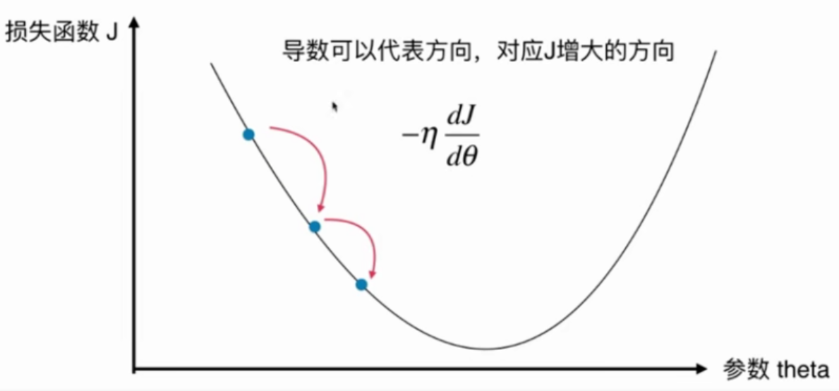
这个二维平面与前面提到的所有二维平面不同。注意坐标系是什么。
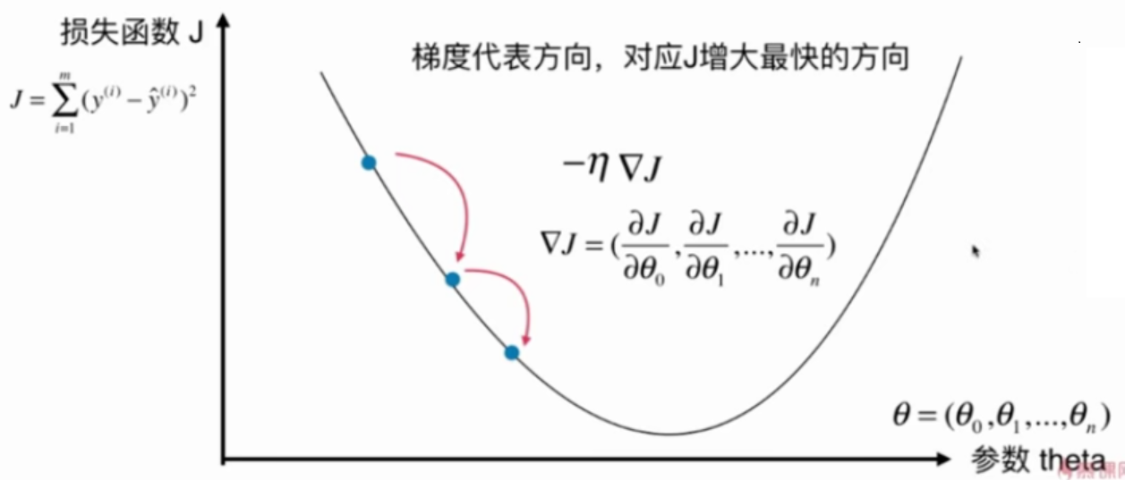
在直线方程中,导数代表斜率
在曲线方程中,导数代表切线斜率
在梯度下降法中,导数代表theta单位变化时,J相应的变化
导数可以代表方向,对应J增大的方向
在梯度下降法中,theta应该向导数的负方向移动
在多维函数中,要对各个方向的分量分别求导,最终得到的方向就是梯度。
注意:并不是所有函数都有唯一的极值点
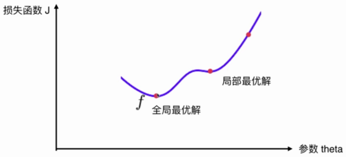
解决方法:
多次运行,随机化初始化点
梯度下降法的初始点也是一个超参数
线性回归问题,损失函数J具有唯一最优解
不是一个机器学习算法
是一种基于搜索的最优化算法
作用:最小化一个损失函数
这个二维平面与前面提到的所有二维平面不同。注意坐标系是什么。
在直线方程中,导数代表斜率
在曲线方程中,导数代表切线斜率
在梯度下降法中,导数代表theta单位变化时,J相应的变化
导数可以代表方向,对应J增大的方向
在梯度下降法中,theta应该向导数的负方向移动
在多维函数中,要对各个方向的分量分别求导,最终得到的方向就是梯度。
注意:并不是所有函数都有唯一的极值点
解决方法:
多次运行,随机化初始化点
梯度下降法的初始点也是一个超参数
线性回归问题,损失函数J具有唯一最优解
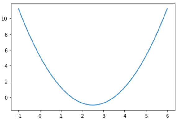
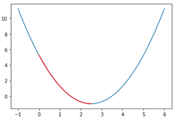
假设损失函数J是这样的:
import numpy as np
import matplotlib.pyplot as plt

plot_x = np.linspace(-1, 6, 141)
plot_y = (plot_x - 2.5) ** 2 -1
plt.plot(plot_x, plot_y)
plt.show()
梯度下降算法实现
def dJ(theta):
    return 2*(theta - 2.5)

def J(theta):
    return (theta-2.5) ** 2 -1

eta = 0.1
epsilon = 1e-8

theta = 0
while True:
    gradient = dJ(theta)
    last_theta = theta
    theta = theta - eta * gradient
    if (abs(J(theta) - J(last_theta)) < epsilon):
        break

print (theta)
print (J(theta))
输出结果:
2.499891109642585
-0.99999998814289
在图是显示所有的theta的轨迹
def gradient_descent(initial_theta, eta, epsilon=1e-8):
    theta = initial_theta
    theta_history = [theta]
    while True:
        gradient = dJ(theta)
        last_theta = theta
        theta = theta - eta * gradient
        theta_history.append(theta)
        #print (theta)
        if (abs(J(theta) - J(last_theta)) < epsilon):
            break
    return theta_history

def plot_theta_history():
    plt.plot(plot_x, J(plot_x))
    plt.plot(np.array(theta_history), J(np.array(theta_history)), color='r')
    plt.show()

eta = 0.01
theta_history = gradient_descent(0., eta)
plot_theta_history()
输出结果:
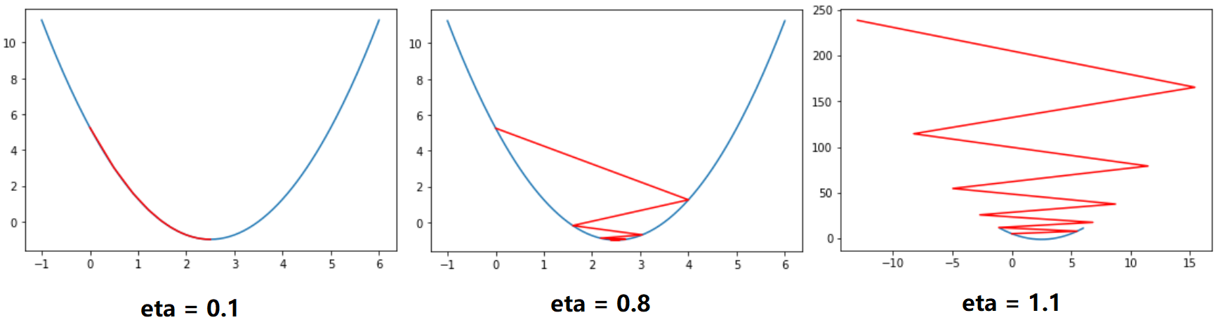
eta取不同参数的绘制结果
def gradient_descent(initial_theta, eta, n_iters = 10, epsilon=1e-8):
    theta = initial_theta
    theta_history = [theta]
    i_iter = 0
    while i_iter < n_iters:
        gradient = dJ(theta)
        last_theta = theta
        theta = theta - eta * gradient
        theta_history.append(theta)
        print (theta)
        if (abs(J(theta) - J(last_theta)) < epsilon):
            break
        i_iter += 1
    return theta_history
输出结果:
import numpy as np
import matplotlib.pyplot as plt

np.random.seed(666)
x = 2 * np.random.random(size=100)
y = x * 3. + 4. + np.random.normal(size=100)

X = x.reshape(-1, 1)

plt.scatter(x, y)
plt.show()
使用梯度下降法训练
def J(theta, X_b, y):
    try:
        return np.sum((y - X_b.dot(theta))**2) / len(X_b)
    except:
        return float('inf')

def dJ(theta, X_b, y):
    ret = np.empty(len(theta))
    ret[0] = np.sum(X_b.dot(theta) - y)
    for i in range(1, len(theta)):
        ret[i] = (X_b.dot(theta) - y).dot(X_b[:, 1])

    return ret * 2 / len(X_b)

def gradient_descent(X_b, y, initial_theta, eta, n_iters = 1e4, epsilon=1e-8):
    theta = initial_theta
    i_iter = 0
    while i_iter < n_iters:
        gradient = dJ(theta, X_b, y)
        last_theta = theta
        theta = theta - eta * gradient
        if (abs(J(theta, X_b, y) - J(last_theta, X_b, y)) < epsilon):
            break
        i_iter += 1
    return theta

X_b = np.hstack([np.ones((len(x), 1)), X])
initial_theta = np.zeros(X_b.shape[1])
eta = 0.01

theta = gradient_descent(X_b, y, initial_theta, eta)
theta
输出结果:
array([4.02145786, 3.00706277])
封装线性回归算法
import numpy as np
from sklearn.metrics import r2_score

class LinearRegression:

    def __init__(self):
        """初始化Linear Regression模型"""
        self.coef_ = None
        self.interception_ = None
        self._theta = None

    def fit_normal(self, X_train, y_train):
        """根据训练数据集X_train, y_train训练Linear Regression模型"""
        assert X_train.shape[0] == y_train.shape[0], "the size of X_train must be equal to the size of y_train"

        X_b = np.hstack([np.ones((len(X_train), 1)), X_train])
        self._theta = np.linalg.inv(X_b.T.dot(X_b)).dot(X_b.T).dot(y_train)

        self.interception_ = self._theta[0]
        self.coef_ = self._theta[1:]

        return self

    def fit_gd(self, X_train, y_train, eta=0.01, n_iters = 1e4):
        """根据训练数据集X_train, y_train,使用梯度下降法训练Linear Regression模型"""
        assert X_train.shape[0] == y_train.shape[0], "the size of X_train must be equal to the size of y_train"

        def J(theta, X_b, y):
            try:
                return np.sum((y - X_b.dot(theta))**2) / len(X_b)
            except:
                return float('inf')

        def dJ(theta, X_b, y):
            ret = np.empty(len(theta))
            ret[0] = np.sum(X_b.dot(theta) - y)
            for i in range(1, len(theta)):
                ret[i] = (X_b.dot(theta) - y).dot(X_b[:, 1])

            return ret * 2 / len(X_b)

        def gradient_descent(X_b, y, initial_theta, eta, n_iters = 1e4, epsilon=1e-8):
            theta = initial_theta
            i_iter = 0
            while i_iter < n_iters:
                gradient = dJ(theta, X_b, y)
                last_theta = theta
                theta = theta - eta * gradient
                if (abs(J(theta, X_b, y) - J(last_theta, X_b, y)) < epsilon):
                    break
                i_iter += 1
            return theta

        X_b = np.hstack([np.ones((len(X_train), 1)), X_train])
        initial_theta = np.zeros(X_b.shape[1])
        self._theta = gradient_descent(X_b, y_train, initial_theta, eta)
        self.interception_ = self._theta[0]
        self.coef_ = self._theta[1:]
        return self

    def predict(self, X_predict):
        """给定待预测数据集X_predict,返回表示X_predict的结果向量"""
        assert self.interception_ is not None and self.coef_ is not None, "must fit before predict"
        assert X_predict.shape[1] == len(self.coef_), "the feature number of X_predict must equal to X_train"

        X_b = np.hstack([np.ones((len(X_predict), 1)), X_predict])
        return X_b.dot(self._theta)

    def score(self, X_test, y_test):
        """根据测试数据集X_test, y_test确定当前模型的准确度"""

        y_predict = self.predict(X_test)
        return r2_score(y_test, y_predict)

    def __repr__(self):
        return "LinearRegression()"
使用fit_gd
lin_reg = LinearRegression()
lin_reg.fit_gd(X, y)
输入:lin_reg.coef_
输出:array([3.00706277])
输入:lin_reg.interception_
输出:4.021457858204859
测试数据
import numpy as np
import matplotlib.pyplot as plt

np.random.seed(666)
x = 2 * np.random.random(size=100)
y = x * 3. + 4. + np.random.normal(size=100)

X = x.reshape(-1, 1)

plt.scatter(x, y)
plt.show()
向量化计算dJ
        def dJ(theta, X_b, y):
            return X_b.T.dot(X_b.dot(theta)-y) * 2. / len(X_b)
使用真实数据测试模型
真实数据 + 正规化方程解
from sklearn.model_selection import train_test_split
X_train, X_test, y_train, y_test = train_test_split(x, y, test_size=0.2, random_state=666)

lin_reg1 = LinearRegression()
lin_reg1.fit_normal(X_train, y_train)  # 见5-4
lin_reg1.score(X_test, y_test)
输出结果:
0.8129794056212832
真实数据 + 梯度下降法
lin_reg2 = LinearRegression()
lin_reg2.fit_gd(X_train, y_train)
lin_reg2.score(X_test, y_test)
输出结果:
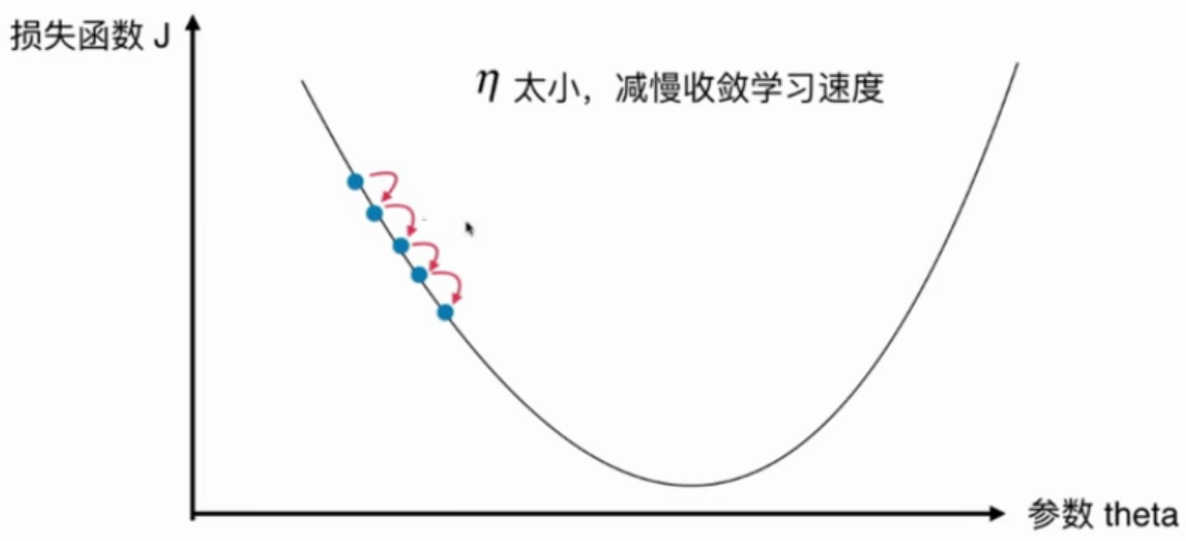
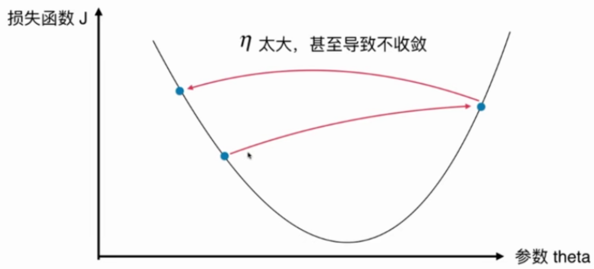
eta太大导致搜索过程不收敛
真实数据 + 梯度下降法 + eta=0.000001
lin_reg2 = LinearRegression()
lin_reg2.fit_gd(X_train, y_train, eta = 0.000001)
lin_reg2.score(X_test, y_test)
输出结果:
0.27586818724477247
训练次数不够,没有达到最优值
真实数据 + 梯度下降法 + eta=0.000001 + n_iters=1e6
lin_reg2 = LinearRegression()
lin_reg2.fit_gd(X_train, y_train, eta = 0.000001, n_iters=1e6)
lin_reg2.score(X_test, y_test)
输出结果:
0.7542932581943915
训练次数太多,导致训练时间太长,但次数又不足以找到最优解
解决方法:数据归一化
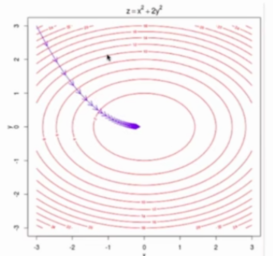
梯度下降法与数据归一化
多元线性回归问题中,不同特征的规格一样,导致eta很难选。同一个eta可能会导致某些无法收敛而另一特征又收敛太慢。
因此使用梯度下降法之前,最好对数据进行归一化
from sklearn.preprocessing import StandardScaler

standardScaler = StandardScaler()
standardScaler.fit(X_train)

X_train_standard = standardScaler.transform(X_train)
X_test_standard = standardScaler.transform(X_test)

lin_reg3 = LinearRegression()
lin_reg3.fit_gd(X_train_standard, y_train)
lin_reg3.score(X_test_standard, y_test)
输出结果:
0.8129873310487505
常规的梯度下降法,又叫批量梯度下降法,Batch Gradient Descent
问题:当样本数m很大时会非常耗时
解决方法:每次只对其中一个样本做计算
把去掉m后计算的公式作为搜索的方向。
由于不能保证这种方法计算得到的方向一定是损失最小的方向,甚至不能保证一定是损失函数减小的方向。也不能找到最小值的位置。
但仍然能到函数的最小值附近。
如果m非常大,可以用一定的精度来换时间。
在随机梯度下降法过程中,学习率很重要。
如果学习率取固定值,很有可以到了最小值附近后又跳出去了。
学习率应逐渐递减。(模拟退火的思想)

通常a取5,b取50
测试数据
import numpy as np
import matplotlib.pyplot as plt

m = 100000

x = np.random.normal(size=m)
X = x.reshape(-1, 1)
y = 4. * x + 3. + np.random.normal(0, 3, size=m)
批量梯度下降法
算法
def J(theta, X_b, y):
    try:
        return np.sum((y - X_b.dot(theta))**2) / len(X_b)
    except:
        return float('inf')

def dJ(theta, X_b, y):
    return X_b.T.dot(X_b.dot(theta)-y) * 2. / len(X_b)

def gradient_descent(X_b, y, initial_theta, eta, n_iters = 1e4, epsilon=1e-8):
    theta = initial_theta
    i_iter = 0
    while i_iter < n_iters:
        gradient = dJ(theta, X_b, y)
        last_theta = theta
        theta = theta - eta * gradient
        if (abs(J(theta, X_b, y) - J(last_theta, X_b, y)) < epsilon):
            break
        i_iter += 1
    return theta
测试性能
%%time
X_b = np.hstack([np.ones((len(X), 1)), X])
initial_theta = np.zeros(X_b.shape[1])
eta = 0.01
theta = gradient_descent(X_b, y, initial_theta, eta)
耗时:2s
theta = array([3.00456203, 3.98777265])
随机梯度下降法
算法
def J(theta, X_b, y):
    try:
        return np.sum((y - X_b.dot(theta))**2) / len(X_b)
    except:
        return float('inf')

def dJ_sgd(theta, X_b_i, y_i):
    return X_b_i.T.dot(X_b_i.dot(theta)-y_i) * 2.

def sgd(X_b, y, initial_theta, n_iters):
    t0 = 5
    t1 = 50

    def learning_rate(t):
        return t0 / (t + t1)

    theta = initial_theta
    i_iter = 0
    for i_iter in range (n_iters):
        rand_i = np.random.randint(len(X_b))
        gradient = dJ_sgd(theta, X_b[rand_i], y[rand_i])
        last_theta = theta
        theta = theta - learning_rate(i_iter) * gradient
        # 不能保证梯度一直是减小的
#         if (abs(J(theta, X_b, y) - J(last_theta, X_b, y)) < epsilon):
#             break
    return theta
测试性能
%%time
X_b = np.hstack([np.ones((len(X), 1)), X])
initial_theta = np.zeros(X_b.shape[1])
theta = sgd(X_b, y, initial_theta, n_iters=len(X_b)//3)   # 这里只检查了1/3样本,对于多元线性回归问题不能这样
耗时:471ms
array([2.94954458, 3.95898273])
时间大幅度减少而结果和批量梯度下降法差不多。
当m特别大时,可以牺牲一定的精度来换取时间。
import numpy as np
from sklearn.metrics import r2_score

class LinearRegression:

    def __init__(self):
        """初始化Linear Regression模型"""
        self.coef_ = None
        self.interception_ = None
        self._theta = None

    def fit_normal(self, X_train, y_train):
        """根据训练数据集X_train, y_train训练Linear Regression模型"""
        assert X_train.shape[0] == y_train.shape[0], "the size of X_train must be equal to the size of y_train"

        X_b = np.hstack([np.ones((len(X_train), 1)), X_train])
        self._theta = np.linalg.inv(X_b.T.dot(X_b)).dot(X_b.T).dot(y_train)

        self.interception_ = self._theta[0]
        self.coef_ = self._theta[1:]

        return self

    def fit_gd(self, X_train, y_train, eta=0.01, n_iters = 1e4):
        """根据训练数据集X_train, y_train,使用梯度下降法训练Linear Regression模型"""
        assert X_train.shape[0] == y_train.shape[0], "the size of X_train must be equal to the size of y_train"

        def J(theta, X_b, y):
            try:
                return np.sum((y - X_b.dot(theta))**2) / len(X_b)
            except:
                return float('inf')

        def dJ(theta, X_b, y):
            return X_b.T.dot(X_b.dot(theta)-y) * 2. / len(X_b)

        def gradient_descent(X_b, y, initial_theta, eta, n_iters = 1e4, epsilon=1e-8):
            theta = initial_theta
            i_iter = 0
            while i_iter < n_iters:
                gradient = dJ(theta, X_b, y)
                last_theta = theta
                theta = theta - eta * gradient
                if (abs(J(theta, X_b, y) - J(last_theta, X_b, y)) < epsilon):
                    break
                i_iter += 1
            return theta

        X_b = np.hstack([np.ones((len(X_train), 1)), X_train])
        initial_theta = np.zeros(X_b.shape[1])
        self._theta = gradient_descent(X_b, y_train, initial_theta, eta)
        self.interception_ = self._theta[0]
        self.coef_ = self._theta[1:]
        return self

    def fit_sgd(self, X_train, y_train, n_iters = 5, t0 = 5, t1 = 50):
        """根据训练数据集X_train, y_train,使用随机梯度下降法训练Linear Regression模型"""
        assert X_train.shape[0] == y_train.shape[0], "the size of X_train must be equal to the size of y_train"

        def dJ_sgd(theta, X_b_i, y_i):
            return X_b_i.T.dot(X_b_i.dot(theta)-y_i) * 2.

        def learning_rate(t, t0, t1):
            return t0 / (t + t1)

        def sgd(X_b, y, initial_theta, n_iters, t0, t1): # n_iters:对所有的样本看几圈
            theta = initial_theta
            m = len(X_b)

            i_iter = 0
            for i_iter in range (n_iters):
                indexes = np.random.permutation(m)
                X_b_new = X_b[indexes]
                y_new = y[indexes]
                for i in range (m):
                    gradient = dJ_sgd(theta, X_b_new[i], y_new[i])
                    last_theta = theta
                    theta = theta - learning_rate(i_iter*m+i, t0, t1) * gradient
            return theta

        X_b = np.hstack([np.ones((len(X_train), 1)), X_train])
        initial_theta = np.zeros(X_b.shape[1])
        self._theta = sgd(X_b, y_train, initial_theta, n_iters, t0, t1)
        self.interception_ = self._theta[0]
        self.coef_ = self._theta[1:]
        return self

    def predict(self, X_predict):
        """给定待预测数据集X_predict,返回表示X_predict的结果向量"""
        assert self.interception_ is not None and self.coef_ is not None, "must fit before predict"
        assert X_predict.shape[1] == len(self.coef_), "the feature number of X_predict must equal to X_train"

        X_b = np.hstack([np.ones((len(X_predict), 1)), X_predict])
        return X_b.dot(self._theta)

    def score(self, X_test, y_test):
        """根据测试数据集X_test, y_test确定当前模型的准确度"""

        y_predict = self.predict(X_test)
        return r2_score(y_test, y_predict)

    def __repr__(self):
        return "LinearRegression()"
测试数据 + sgd
m = 100000

x = np.random.normal(size=m)
X = x.reshape(-1, 1)
y = 4. * x + 3. + np.random.normal(0, 3, size=m)

lin_reg = LinearRegression()
lin_reg.fit_sgd(X, y, n_iters=2)
刚开始在代码中犯了个错误,没有把L78的i_iter改成i_iter*m+i,
导致每次训练得到的模型差点都非常大,且偏离正确值也非常大。
改掉之后就好了,
可以如果学习率使用固定值,不能得到很好的效果。
真实数据 + sgd
真实数据
from sklearn import datasets

boston = datasets.load_boston()
X = boston.data
y = boston.target

X = X[y<50.0]
y = y[y<50.0]
预处理
from sklearn.model_selection import train_test_split
X_train, X_test, y_train, y_test = train_test_split(X, y, test_size=0.2, random_state=666)

from sklearn.preprocessing import StandardScaler
standScaler = StandardScaler()
standScaler.fit(X_train)
X_train_standard = standScaler.transform(X_train)
X_test_standard = standScaler.transform(X_test)
SGD
lin_reg = LinearRegression()
%time lin_reg.fit_sgd(X_train_standard, y_train)
lin_reg.score(X_test_standard, y_test)
n_iters对score和Wall time的影响
| n_iters | score | Wall time |
|---|---|---|
| 5 | 0.7763594773981595 | 30.7 ms |
| 50 | 0.8130771495096732 | 271 ms |
| 100 | 0.8131205440883096 | 462 ms |
真实数据 + sklearn的SGD
from sklearn.linear_model import SGDRegressor

sgd_lin = SGDRegressor()
%time sgd_lin.fit(X_train_standard, y_train)
sgd_lin.score(X_test_standard, y_test)
模型的得分差不多,但sklearn的SGD的速度明显快很多。
因为sklearn的SGD的实现过程与课程中有很大的不同。
视频还测试了SGDRegressor的n_iter参数。
这个参数在我用的sklearn版本中已经没有了。
梯度的求解并不容易,如果知道自己求的梯度是否正确?

图中两条直线的斜率近乎相等。
两个蓝点越接近,斜率越相近。
推广到高维场景
代码实现
准备数据
import numpy as np
import matplotlib.pyplot as plt

np.random.seed(666)
X = np.random.random(size=(1000, 10))
true_theta = np.arange(1, 12, dtype=float)
X_b = np.hstack([np.ones((len(X), 1)), X])
y = X_b.dot(true_theta) + np.random.normal(size=1000)

def J(theta, X_b, y):
    try:
        return np.sum((y - X_b.dot(theta))**2) / len(X_b)
    except:
        return float('inf')
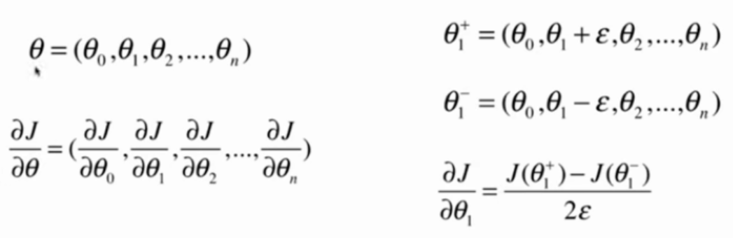
两种方法求导数
def dJ_math(theta, X_b, y):
    return X_b.T.dot(X_b.dot(theta) - y) * 2. / len(y)

def dJ_debug(theta, X_b, y, epsilon=0.01):
    ret = np.empty(len(theta))
    for i in range(len(theta)):
        theta_1 = theta.copy()
        theta_1[i] +=epsilon
        theta_2 = theta.copy()
        theta_2[i] -=epsilon
        ret[i] = (J(theta_1, X_b, y) - J(theta_2, X_b, y)) / (2*epsilon)
    return ret
两种方法训练模型
def gradient_descent(dJ, X_b, y, initial_theta, eta, n_iters = 1e4, epsilon=1e-8):
    theta = initial_theta
    i_iter = 0
    while i_iter < n_iters:
        gradient = dJ(theta, X_b, y)
        last_theta = theta
        theta = theta - eta * gradient
        if (abs(J(theta, X_b, y) - J(last_theta, X_b, y)) < epsilon):
            break
        i_iter += 1
    return theta

X_b = np.hstack([np.ones((len(X), 1)), X])
initial_theta = np.zeros(X_b.shape[1])
eta = 0.01

%time theta = gradient_descent(dJ_debug, X_b, y, initial_theta, eta)
%time theta = gradient_descent(dJ_math, X_b, y, initial_theta, eta)
实验结果
dJ_math对应的运行时间为:660 ms
dJ_debug对应的运行时间为:4.58s
两种方法求出的theta完全相同
dJ_debug的方法可以用于求梯度,最终能得到正确的结果
dJ_debug速度很慢。
可以先使用dJ_debug得到想要的正确结果。
再用dJ_math将得到的结果与dJ_debug的结果相比较,来验证数学是否正确。
dJ_debug与J无关,可以适用于所有函数。
- 批量梯度下降法 Batch Gradient Descent,缺点:慢,优点:稳定
- 随机梯度下降法 Stochastic Gradient Descent,优点:快,缺点:不稳定
- 小批量梯度下降法 Mini-Batch Gradient Descent,以上两种结合
随机
随机梯度下降法可以跳出局部最优解
随机梯度下降法运行速度更快
机器学习领域很多算法都要使用随机的特点,例如随机搜索、随机森林
主成分分析法 PCA Principal Component Analysis
一个非监督的机器学习算法
主要用于数据的降维
通过降维,可以发现更便于人类理解的特征
其他应用:可视化,去噪
主成分分析法 PCA Principal Component Analysis
一个非监督的机器学习算法
主要用于数据的降维
通过降维,可以发现更便于人类理解的特征
其他应用:可视化,去噪
二维降至一维
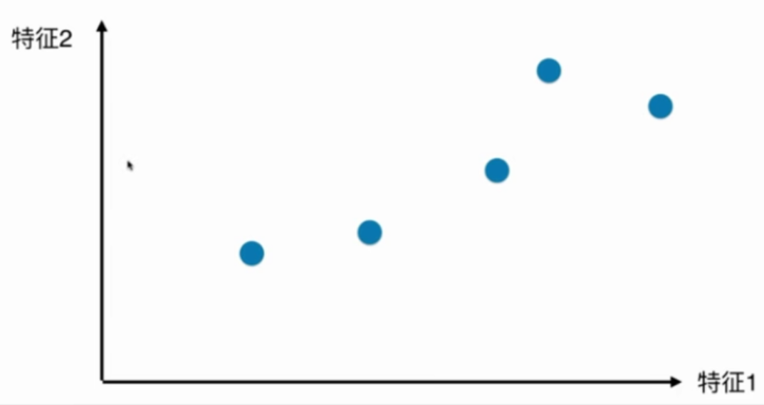
如何把图中的二维空间中的点降至一维?

以上三种方法哪种更好?
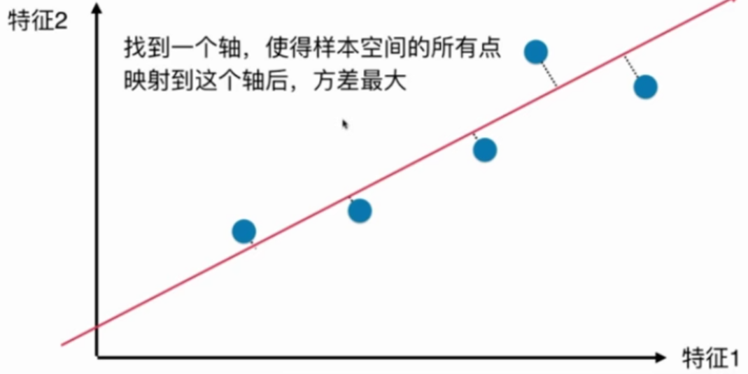
第三种,因为第三种最大程度地保留了原数据之间的关系.
概率论与数理统计中, 方差(Variance)描述了样本整体疏密的一个指标.
如何找到这个样本间间距(方差)最大的轴?
$$ \begin{aligned} Var(x) = \frac{1}{m}\sum_{i=1}^m(x_i-\bar x)^2 && (1) \end{aligned} $$
其中 $$\bar x$$ 代表x的平均值。
第一步:将所有样本的均值归0 (demean)

由于均值为0,则公式(1)可以化简为:
$$ \begin{aligned} Var(x) = \frac{1}{m}\sum_{i=1}^m(x_i-\bar x)^2 = \frac{1}{m}\sum_{i=1}^mx_i^2 && (2) \end{aligned} $$
这里的x是样本映射到坐标轴以后的新的样本的值 $$X_{\text{project}}$$ 。
第二步:求一个轴的方向w = (w1, w2),使用所有的样本映射到w以后,有 $$Var(X_{\text{project}})$$ 最大:
$$ \begin{aligned} Var(X_{\text{project}}) = \frac{1}{m}\sum_{i=1}^m||x^{(i)}_{\text{project}}||^2 && (3) \end{aligned} $$
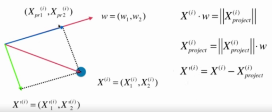
推导过程:
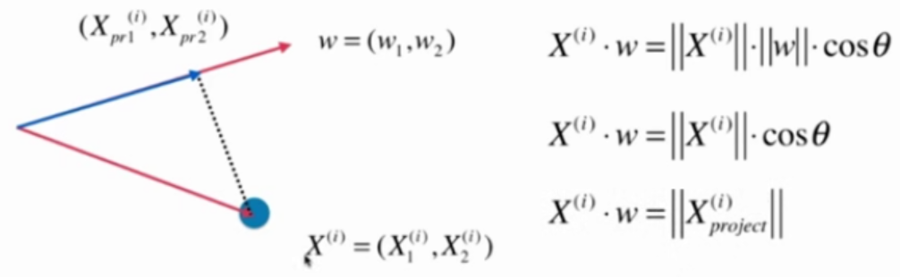
假设均值化之后的x的坐标为
$$ X^{(i)}=(X^{(i)}_1, X^{(i)}_2) $$
要映射的坐标轴为 $$w-{w_1, w_2}$$
$$X^{(i)}$$ 映射到 $$w - {w_1, w_2}$$ 之后的新坐标为
$$X_{pr}^{(i)} = (X^{(i)}{pr1}, X^{(i)}{pr2})$$
那么, $$||x^{(i)}_{\text{project}}||$$ 为:
$$ ||x^{(i)}_{\text{project}}|| = X^{(i)} \cdot w $$
代入公式(3)得:
$$ \begin{aligned} Var(X_{\text{project}}) = \frac{1}{m}\sum_{i=1}^m|| X^{(i)} \cdot w||^2 && (4) \end{aligned} $$
目标是最大化公式(4),这是一个求目标函数的最优化问题,使用梯度上升法解决。
主成分分析法和线性回归的区别
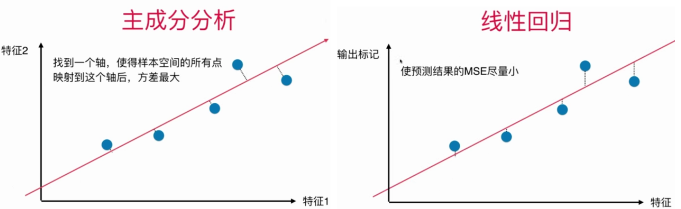
| 主成分分析 | 线性回归 --|---|-- 坐标轴 | 2个特征 | 1个特征和输出标记 要求的是什么 | 一个方向 | 一根直线 经过点的线与什么垂直 | 所求的方向垂直 | x轴 目标 | 方差最大 | MSE最小
 这是一个非监督学习算法,在式子中没有输出标记y
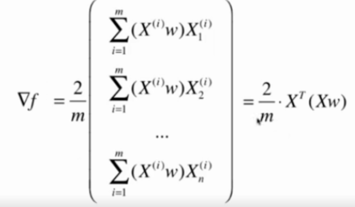
使用梯度上升法,就要先对目标函数求梯度,计算结果如下:
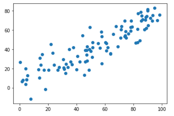
import numpy as np
import matplotlib.pyplot as plt

X = np.empty((100, 2))
X[:,0] = np.random.uniform(0., 100, size=100)
X[:,1] = 0.75 * X[:, 0] + 3. + np.random.normal(0, 10., size=100)

plt.scatter(X[:,0], X[:,1])
plt.show()
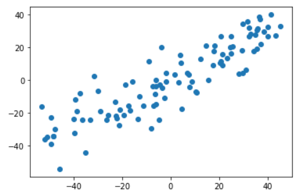
第一步:demean
def demean(X):
    return X - np.mean(X, axis=0)

X_demean = demean(X)
plt.scatter(X_demean[:,0], X_demean[:,1])
plt.show()
第二步:梯度上升法
def f(w, X):
    return np.sum((X.dot(w)**2)) / len(X)

def df_math(w, X):
    return X.T.dot(X.dot(w)) * 2. / len(X)

def df_debug(w, X, epsilon=0.0001):
    res = np.empty(len(w))
    for i in range(len(w)):
        w_1 = w.copy()
        w_1[i] += epsilon
        w_2 = w.copy()
        w_2[i] -= epsilon
        res[i] = (f(w_1, X) - f(w_2, X)) / (2 * epsilon)
    return res

# 把向量单位化
def direction(w):
    return w / np.linalg.norm(w)

def gradient_ascent(df, X, initial_w, eta, n_iters=1e4, epsilon=1e-8):
    w = direction(initial_w)
    cur_iter = 0
    while cur_iter < n_iters:
        gradient = df(w, X)
        last_w = w
        w = w + eta * gradient
        w = direction(w)
        if(abs(f(w, X)) - abs(f(last_w, X)) < epsilon):
           break
        cur_iter += 1
    return w
注意1:epsilon取值比较小,因为w是方向向量,它的每个维度都很小,所以epsilon也要取很小的值
注意2:每次计算出w后要对其单位化
如果每次计算出w后不做单位化的工作,算法也可以工作,因为w本身也是代方向的。
但这样会导致搜索过程不顺畅。
因为如果不做单位化,w应该是公式要求的w偏大的,这就要求eta值非常小。
而eta值小又会导致循环次数非常多,性能就会下降。
因此遵循公式的假设条件,每次都让w成为方向向量。
训练和绘制结果
initial_w = np.random.random(X.shape[1])
eta = 0.001
gradient_ascent(df_debug, X_demean, initial_w, eta)
w = gradient_ascent(df_math, X_demean, initial_w, eta)
plt.scatter(X_demean[:, 0], X_demean[:, 1])
plt.plot([0, w[0]*30], [0, w[1]*30], color='r')
plt.show()

注意3:w不能是零向量。因为w=0本身也是在极值点上,是极小值点,此时梯度也会0
注意4:不能使用StandardScaler标准化数据。
因为本算法的目标就是让方差最大。
一但对数据做了标准化,样本的方差就肯定是1了,不存在方差最大值。
另一个更极端的例子
X2 = np.empty((100, 2))
X2[:,0] = np.random.uniform(0., 100, size=100)
X2[:,1] = 0.75 * X2[:, 0] + 3.

X2_demean = demean(X2)
w2 = gradient_ascent(df_debug, X2_demean, initial_w, eta)

plt.scatter(X2_demean[:, 0], X2_demean[:, 1])
plt.plot([0, w2[0]*30], [0, w2[1]*30], color='r')
plt.show()
本质上是从一组坐标第转移到了另一组坐标系。 原来的坐标系有n个方向,那么新的坐标系也应该有n个方向。 7-2中的算法只是求出第一个轴的方向。
在新的坐标系中,第一个轴保存了样本最大的方差,称为第一个主成分。 第二个次之,依此类推。
问:求出第一主成分以后,如何求出下一主成分呢?
答:
第一步: 改变数据,将数据的第一个主成分去掉。
图中X'是X去除了第一主成分上的分量后的结果
第二步: 在新数据上求第一主成分
准备数据
import numpy as np
import matplotlib.pyplot as plt

X = np.empty((100, 2))
X[:,0] = np.random.uniform(0., 100, size=100)
X[:,1] = 0.75 * X[:, 0] + 3. + np.random.normal(0, 10., size=100)

plt.scatter(X[:,0], X[:,1])
plt.show()
第一步:demean
def demean(X):
    return X - np.mean(X, axis=0)

X_demean = demean(X)
plt.scatter(X_demean[:,0], X_demean[:,1])
plt.show()
第二步:梯度上升法
def f(w, X):
    return np.sum((X.dot(w)**2)) / len(X)

def df(w, X):
    return X.T.dot(X.dot(w)) * 2. / len(X)

# 把向量单位化
def direction(w):
    return w / np.linalg.norm(w)

def first_component(X, initial_w, eta, n_iters=1e4, epsilon=1e-8):
    w = direction(initial_w)
    cur_iter = 0
    while cur_iter < n_iters:
        gradient = df(w, X)
        last_w = w
        w = w + eta * gradient
        w = direction(w)
        if(abs(f(w, X)) - abs(f(last_w, X)) < epsilon):
           break
        cur_iter += 1
    return w
训练和绘制结果
initial_w = np.random.random(X.shape[1])
eta = 0.001
w = first_component(X_demean, initial_w, eta)
输入:w
输出:array([0.77135006, 0.63641109])
第三步:去掉第一个主成分
方法一:
X2 = np.empty(X.shape)
for i in range(len(X)):
   X2[i] = X[i] - X[i].dot(w) * w
方法二:
X2 = X - X.dot(w).reshape(-1, 1) * w
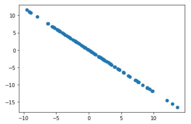
去掉第一主成分后的数据
plt.scatter(X2[:,0], X2[:,1])
plt.show()
第四步:求新数据的第一主成分
w2 = first_component(X2, initial_w, eta)
输入:w2
输出:array([-0.63639346, 0.77136461])
输入:w.dot(w2)
输出:2.2857453091384983e-05
点乘结果几乎为0,说明w和w2是垂直关系
封装成函数
def first_n_component(n, X, eta = 0.01, n_iters=1e4, epsilon=1e-8):
    X_pca = X.copy()
    X_pca = demean(X_pca)
    res = []
    for i in range(n):
        initial_w = np.random.random(X.shape[1])
        eta = 0.001
        w = first_component(X_pca, initial_w, eta)
        res.append(w)
        X_pca = X_pca - X_pca.dot(w).reshape(-1, 1) * w
    return res
输入:first_n_component(2, X)
输出:[array([0.77135082, 0.63641018]), array([ 0.63642749, -0.77133653])]
[?]遗留问题:我算出的第二个主成分的方向和视频中是反的?
可能是跟initial_w有关,多次运行后发现两个方向的结果都有。
定义:X是样本数据,每一行是一个数据,它有m个数据,每个数据有n个特征
$$
X =
\begin{bmatrix}
X_1^{(1)} && X_1^{(2)} && \cdots && X_1^{(n)} \
X_2^{(1)} && X_2^{(2)} && \cdots && X_2^{(n)} \
\cdots && \cdots && \cdots && \cdots \
X_m^{(1)} && X_m^{(2)} && \cdots && X_m^{(n)}
\end{bmatrix}
$$
$W_k$是求得的前k个主成分矩阵,每一行是一个主成分的单位方向,它有k个主成分方向,每个主成分的方向有n个维度
$$
X =
\begin{bmatrix}
W_k^{(1)} && W_1^{(2)} && \cdots && W_1^{(n)} \
W_2^{(1)} && W_2^{(2)} && \cdots && W_2^{(n)} \
\cdots && \cdots && \cdots && \cdots \
W_k^{(1)} && W_k^{(2)} && \cdots && W_k^{(n)}
\end{bmatrix}
$$
问:如何将样本X从N维转换成K维?
答:降维:把所有样本映射到K个主成分上
$$
X \cdot W_k^T = X_k
$$
还原:把降维后的数据还原到原坐标空间
$$
X_k \cdot W_k = X_m
$$
还原后的X与原X不同。
把PCA封装成类
import numpy as np

class PCA:
    def __init__(self, n_components):
        """初始化PCA"""
        assert n_components >= 1, "n_components must be valid"
        self.n_components = n_components
        self.components_ = None

    def fit(self, X, eta=0.01, n_iters=1e4):
        """获取数据集的前n个主成分"""
        assert self.n_components <= X.shape[1], "n_components must not be greater than the feature number of X"

        def demean(X):
            return X - np.mean(X, axis=0)

        def f(w, X):
            return np.sum((X.dot(w)**2)) / len(X)

        def df(w, X):
            return X.T.dot(X.dot(w)) * 2. / len(X)

        # 把向量单位化
        def direction(w):
            return w / np.linalg.norm(w)

        def first_component(X, initial_w, eta, n_iters=1e4, epsilon=1e-8):
            w = direction(initial_w)
            cur_iter = 0
            while cur_iter < n_iters:
                gradient = df(w, X)
                last_w = w
                w = w + eta * gradient
                w = direction(w)
                if(abs(f(w, X)) - abs(f(last_w, X)) < epsilon):
                   break
                cur_iter += 1
            return w

        X_pca = demean(X)
        self.components_ = np.empty(shape = (self.n_components, X.shape[1]))
        for i in range(self.n_components):
            initial_w = np.random.random(X.shape[1])
            eta = 0.001
            w = first_component(X_pca, initial_w, eta)
            self.components_[i, :] = w
            X_pca = X_pca - X_pca.dot(w).reshape(-1, 1) * w
        return self

    def transform(self, X):
        """将给定的X,映射到各个主成分分量中"""
        assert X.shape[1] == self.components_.shape[1]
        return X.dot(self.components_.T)

    def inverse_transform(self, X):
        """将给定的X反向映射回原来的特征空间"""
        assert X.shape[1] == self.components_.shape[0]
        return X.dot(self.components_)

    def __repr__(self):
        return "PCA(n_components=%d)" % self.n_components
使用PCA降维
准备数据
import numpy as np
import matplotlib.pyplot as plt

X = np.empty((100,2))
X[:,0] = np.random.uniform(0., 100., size=100)
X[:,1] = 0.75 * X[:, 0] + 3. + np.random.normal(0, 10., size=100)
训练模型1
pca = PCA(n_components=2)
pca.fit(X)
输入:pca.components_
输出:array([[ 0.75366776, 0.65725559], [-0.65723751, 0.75368352]])
训练模型2:降维
pca = PCA(n_components=1)
pca.fit(X)

X_reduction = pca.transform(X)
X_restore = pca.inverse_transform(X_reduction)
输入:X_reduction.shape
输出:(100, 1)
输入:X_restore.shape
输出:(100, 2)
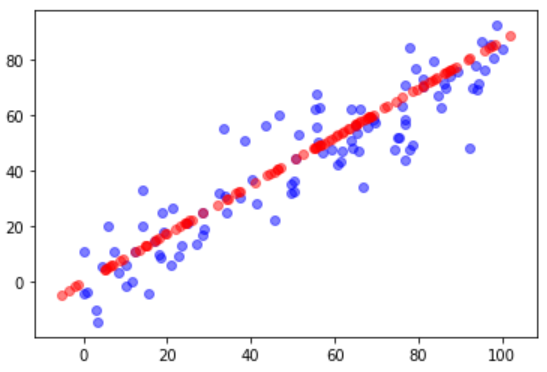
对比原始数据与降维再恢复后的数据
plt.scatter(X[:, 0], X[:, 1], color='b', alpha=0.5)
plt.scatter(X_restore[:, 0], X_restore[:, 1], color='r', alpha=0.5)
plt.show()
沿用7-5中的测试数据,使用scikit-learn中的PCA
from sklearn.decomposition import PCA

pca = PCA(n_components=1)
pca.fit(X)
输入:pca.components_
输出:array([[-0.75366744, -0.65725595]])
这个轴与7-5中的计算结果是相反的。因为scikit-learn中不是什么梯度下降法而是什么数学方法计算的。
轴的方向相反不影响算法的结果
对比原始数据与降维再恢复后的数据
X_reduction = pca.transform(X)
X_restore = pca.inverse_transform(X_reduction)

plt.scatter(X[:, 0], X[:, 1], color='b', alpha=0.5)
plt.scatter(X_restore[:, 0], X_restore[:, 1], color='r', alpha=0.5)
plt.show()
使用真实数据测试PCA降维对效率和准确度的影响
真实数据
import numpy as np
import matplotlib.pyplot as plt
from sklearn import datasets

digits = datasets.load_digits()
X = digits.data
y = digits.target

from sklearn.model_selection import train_test_split
X_train, X_test, y_train, y_test = train_test_split(X, y, random_state=666)
几种降维结果比较
| PCA后的维数 | 运行时间 | score |
|---|---|---|
| 不降维 | 82.9 ms | 0.9866666666666667 |
| 2 | 2.2 | 0.6066666666666667 |
| 28 | 1,05 时间更少了? | 0.98 |
结论: 如果n_components选择合适,会大大减少训练时间而略微减少分类准确度,这样做是值得的。
选择合适的降维效果
确定新坐标系中每个维度保存了原数据的方差百分比
pca = PCA(n_components=X_train.shape[1])
pca.fit(X_train)
pca.explained_variance_ratio_
输出结果:
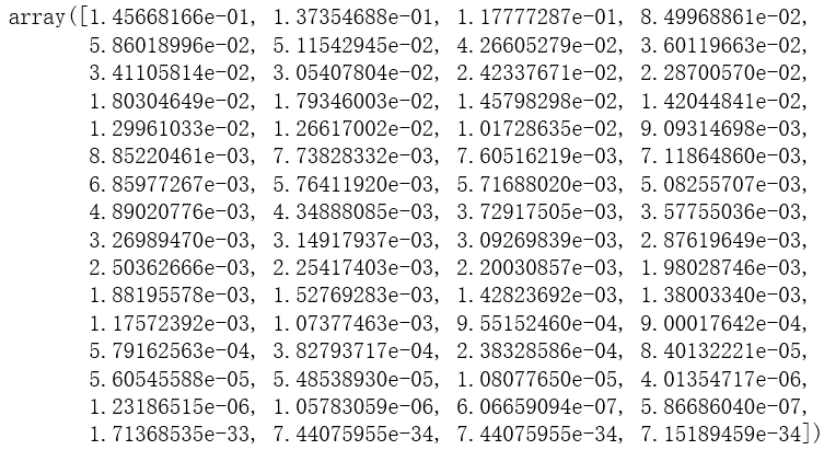
plt.plot([i for i in range(X_train.shape[1])],
    [np.sum(pca.explained_variance_ratio_[:i+1]) for  i in range(X_train.shape[1])])
plt.show()
输出结果:
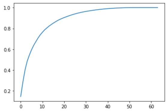
这张图表示了前N个维度所占方差的百分比
保留原始数据95%的方差
pca = PCA(0.95)
pca.fit(X_train)
pca.explained_variance_ratio_
对原始数据降至2维的结果也有一定参考意义
pca = PCA(n_components=2)
pca.fit(X)
X_reduction = pca.transform(X)

for i in range(10):
    plt.scatter(X_reduction[y==i, 0], X_reduction[y==i,1], alpha=0.8)
plt.show()

假如只是要区分图中紫色的数据和红色的数据,降到2维就足够了
使用sklearn提供的接口加载经典的MNIST手写数据集
import numpy as np
from sklearn.datasets import fetch_openml

mnist_data = fetch_openml("mnist_784")

X, y = mnist_data['data'], mnist_data['target']     # X.shape = (70000, 784)
X_train = np.array(X[:60000], dtype=float)
y_train = np.array(y[:60000], dtype=float)
X_test = np.array(X[60000:], dtype=float)
y_test = np.array(y[60000:], dtype=float)
KNN算法对MNIST分类
from sklearn.neighbors import KNeighborsClassifier

knn_clf = KNeighborsClassifier()
%time knn_clf.fit(X_train, y_train)   # Wall time: 1min 3s

%time knn_clf.score(X_test, y_test)   # Wall time = 15min 43, score = 0.9688
Note 1:
为什么KNN算法的fit要花费这么多时间?
因为当训练数据比较大的情况下,sklearn的KNN算法会使用tree来存储数据,而不是直接存储数据。
Note 2:
KNN算法通常需要对数据进行归一化,为什么这里没有做归一化?
因为当前的样本数据中,所有的特征都是表示图像中的像素点,整体处于同一个尺度,所以不需要归一化。
Note 3:
训练样本非常大的情况下,KNN算法非常耗时
PCA + KNN + MNIST
from sklearn.decomposition import PCA

pca = PCA(0.9)
pca.fit(X_train)
X_train_reduction = pca.transform(X_train)   # X_train_reductionduction.shape = (60000, 784)

knn_clf = KNeighborsClassifier()
%time knn_clf.fit(X_train_reduction, y_train)   # Wall time: 15.6 s

X_test_reduction = pca.transform(X_test)
%time knn_clf.score(X_test_reduction, y_test)   # Wall time = 2min 20s, score = 0.8728
运行时间减少的同时,预测准确率反面提高了
PCA在降维的同时还可以降噪
之前的例子
原始数据:
import numpy as np
import matplotlib.pyplot as plt

X = np.empty((100,2))
X[:,0] = np.random.uniform(0., 100., size=100)
X[:,1] = 0.75 * X[:,0] + 3. + np.random.normal(0, 5, size=100)

plt.scatter(X[:, 0], X[:, 1])
plt.show()

降噪后:
from sklearn.decomposition import PCA
pca = PCA(n_components=1)
pca.fit(X)
X_reduction = pca.transform(X)
X_restore = pca.inverse_transform(X_reduction)
plt.scatter(X_restore[:, 0], X_restore[:, 1])
plt.show()

从图1到图2有信丢失了,丢失的这部分信息中很有可能有很大一部分是噪声 降维的过程中丢失了信息,同时也去除了部分噪音
手写识别例子
原始的手写数据:
from sklearn import datasets

digits = datasets.load_digits()
X = digits.data
y = digits.target

example_digits = X[y == 0, :][:10]
for num in range(1, 10):
    X_num = X[y==num,:][:10]
    example_digits = np.vstack([example_digits, X_num])
对原始的手写数据加噪
example_digits = example_digits + np.random.normal(0, 4, size=X.shape)
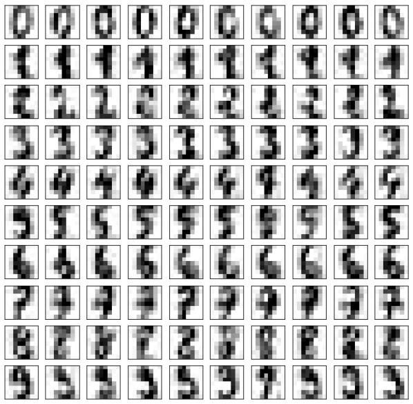
显示加噪后的图像:
def plot_digits(data):
    #fig, axes = plt.subplots(10, 10, figsize=(10, 10), subplot_kw={'xticks':[], 'yticks':[]},girdspec_kw=dict(hspace=0.1, wspace=0.1))
    fig, axes = plt.subplots(10, 10, figsize=(10, 10), subplot_kw={'xticks':[], 'yticks':[]})
    for i,ax in enumerate(axes.flat):
        ax.imshow(data[i].reshape(8, 8), cmap='binary', interpolation='nearest', clim=(0,16))
    plt.show()

plot_digits(example_digits)

对example_digits去噪
pca = PCA(0.5)
pca.fit(noisy_digits)   # pca.n_components_ = 12
components = pca.transform(example_digits)
filtered_digits = pca.inverse_transform(components)
去噪后的效果:
plot_digits(filtered_digits)

把W矩阵中的每一行看作一个方向,第一行代表最重要的方向,第二行代表次重要的方向,依次类推
也可以说:
将W矩阵中的每一行看作一个样本,第一行所代表的样本是最重要的样本,最能反应原X矩阵样本特征的样本。第二行所代表的样本是次重要的样本,依次类推。
X中的每一行都是一张人脸,W中的每一行也可以认为是一张脸,称为特征脸。每一个特征脸都是一个主成分,相当于表达了原样本数据的特征。(特征这个词与矩阵中的特征值这个词相对应)
取数据
import numpy as np
import matplotlib.pyplot as plt
from sklearn.datasets import fetch_lfw_people

faces = fetch_lfw_people()
random_indexes = np.random.permutation(len(faces.data))
X = faces.data[random_indexes]
查看图像:
def plot_faces(faces):
    #fig, axes = plt.subplots(6, 6, figsize=(10, 10), subplot_kw={'xticks':[], 'yticks':[]},girdspec_kw=dict(hspace=0.1, wspace=0.1))
    fig, axes = plt.subplots(10, 10, figsize=(10, 10), subplot_kw={'xticks':[], 'yticks':[]})
    for i,ax in enumerate(axes.flat):
        ax.imshow(data[i].reshape(62, 47), cmap='bone')
    plt.show()

plot_faces(example_faces)
特征脸
from sklearn.decomposition import PCA
pca = PCA(svd_solver="randomized")  #因为数据样本比较大,用随机的方式会快一些

%timeit pca.fit(X)

plot_faces(pca.components_[:36, :])
其它关于样本库
faces2 = fetch_lfw_people(min_faces_per_person=60) # 取一个人至少有60张照片的样本
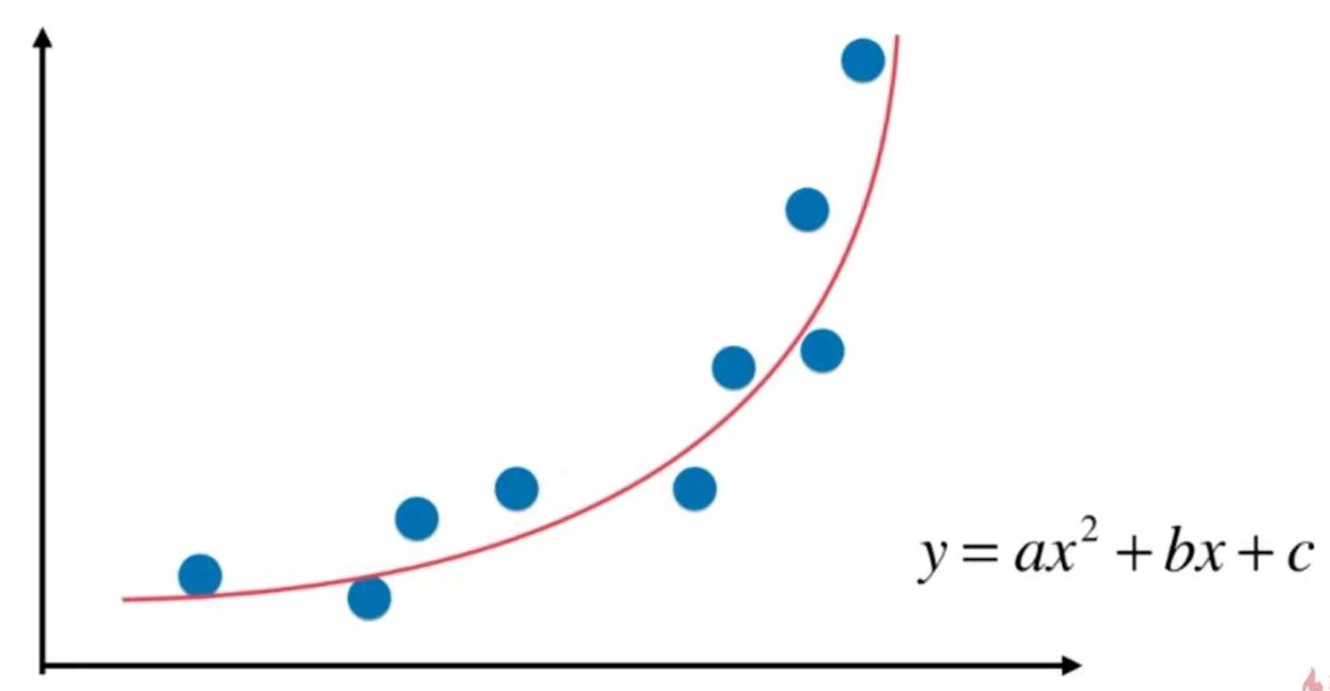
线性回归要求数据存在线性关系。
但实际场景中,存在强线性关系的数据是比较少的,大部分情况下数据之间是非线性关系。
用一种简单的手段改进线性回归法,使得它可以处理和预测非线性数据。
即多项式回归。
准备数据
import numpy as np
import matplotlib.pyplot as plt
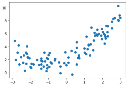
x = np.random.uniform(-3, 3, size=100)
X = x. reshape(-1, 1)
y = 0.5 * x**2 + x + 2 + np.random.normal(0, 1, size=100)
plt.scatter(X, y)
plt.show()
使用线性回归
from sklearn.linear_model import LinearRegression

lin_reg = LinearRegression()
lin_reg.fit(X, y)
y_predict = lin_reg.predict(X)

plt.scatter(x, y)
plt.plot(x, y_predict, color='r')
plt.show()

解决方案, 添加一个特征
X2 = np.hstack([X, X**2])

lin_reg2 = LinearRegression()
lin_reg2.fit(X2, y)
y_predict2 = lin_reg2.predict(X2)

plt.scatter(x, y)
plt.plot(np.sort(x), y_predict2[np.argsort(x)], color='r')
plt.show()
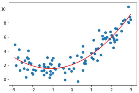
看上去这根曲线拟合得更好。
输入:lin_reg2.coef_
输出:array([0.99902653, 0.46334749])
0.999是x的系数,0.46是x^2的系数
输入:lin_reg2.intercept_
输出:2.0518267069340164
结论
使用线性回归的思路,为原来的样本添加新的特征,新的特征是原有特征的多项式的组合。以此来解决非线性问题。
PCA是对数据做降维处理,这里则是对数据集升维。通过升维和添加特征,使算法拟合高维度的数据。
线性回归要求数据存在线性关系。
但实际场景中,存在强线性关系的数据是比较少的,大部分情况下数据之间是非线性关系。
用一种简单的手段改进线性回归法,使得它可以处理和预测非线性数据。
即多项式回归。
准备数据
import numpy as np
import matplotlib.pyplot as plt

x = np.random.uniform(-3, 3, size=100)
X = x. reshape(-1, 1)
y = 0.5 * x**2 + x + 2 + np.random.normal(0, 1, size=100)

plt.scatter(X, y)
plt.show()
使用线性回归
from sklearn.linear_model import LinearRegression

lin_reg = LinearRegression()
lin_reg.fit(X, y)
y_predict = lin_reg.predict(X)

plt.scatter(x, y)
plt.plot(x, y_predict, color='r')
plt.show()
解决方案, 添加一个特征
X2 = np.hstack([X, X**2])

lin_reg2 = LinearRegression()
lin_reg2.fit(X2, y)
y_predict2 = lin_reg2.predict(X2)

plt.scatter(x, y)
plt.plot(np.sort(x), y_predict2[np.argsort(x)], color='r')
plt.show()
看上去这根曲线拟合得更好。
输入:lin_reg2.coef_
输出:array([0.99902653, 0.46334749])
0.999是x的系数,0.46是x^2的系数
输入:lin_reg2.intercept_
输出:2.0518267069340164
结论
使用线性回归的思路,为原来的样本添加新的特征,新的特征是原有特征的多项式的组合。以此来解决非线性问题。
PCA是对数据做降维处理,这里则是对数据集升维。通过升维和添加特征,使算法拟合高维度的数据。
准备数据
import numpy as np
import matplotlib.pyplot as plt

x = np.random.uniform(-3, 3, size=100)
X = x. reshape(-1, 1)
y = 0.5 * x**2 + x + 2 + np.random.normal(0, 1, size=100)
使用polynomialFeatures为原数据升维
from sklearn.preprocessing import PolynomialFeatures
poly = PolynomialFeatures(degree=2)
poly.fit(X)
X2 = poly.transform(X)
输入:X2.shape
输出:(100, 3)
输入:X2[:5,:]
输出:
array([[ 1.        , -1.34284888,  1.80324311],
       [ 1.        , -0.18985858,  0.03604628],
       [ 1.        , -1.58563134,  2.51422675],
       [ 1.        ,  1.2149354 ,  1.47606802],
       [ 1.        , -2.05874706,  4.23843944]])
输入:X2[:5,:]
输出:
array([[-1.34284888],
       [-0.18985858],
       [-1.58563134],
       [ 1.2149354 ],
       [-2.05874706]])
X2中第一列是1,第二列是原数据,第三列是原数据的平方
使用scikit-learn中的线性回归算法
这一部分与8-1相同
from sklearn.linear_model import LinearRegression

lin_reg2 = LinearRegression()
lin_reg2.fit(X2, y)
y_predict2 = lin_reg2.predict(X2)

plt.scatter(x, y)
plt.plot(np.sort(x), y_predict2[np.argsort(x)], color='r')
plt.show()
输入:lin_reg2.coef_
输出:array([0. , 1.01723515, 0.46407147])
0是对X2是第一列数据拟合的结果
输入:lin_reg2.intercept_
输出:2.1789150996943945
关于PolynomialFeatures
X = np.arange(1,11).reshape(-1, 2)
poly = PolynomialFeatures(degree=2)
poly.fit(X)
X2 = poly.transform(X)
输入:X.shape
输出:(5, 2)
输入:X
输出:array([[ 1, 2], [ 3, 4], [ 5, 6], [ 7, 8], [ 9, 10]])
输入:X2.shape
输出:(5, 6)
输入:X2
输出:
array([[  1.,   1.,   2.,   1.,   2.,   4.],
       [  1.,   3.,   4.,   9.,  12.,  16.],
       [  1.,   5.,   6.,  25.,  30.,  36.],
       [  1.,   7.,   8.,  49.,  56.,  64.],
       [  1.,   9.,  10.,  81.,  90., 100.]])
第一列:1,即0次幂
第二列:x1,1次幂
第三列:x2,1次幂
第四列:x1^2,2次幂
第五列:x1*x2,2次幂
第六列:x2^2,2次幂
假设有x1, x2两个特征,PolynomialFeatures(degree=3),会得到多少项数据?
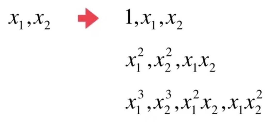
poly = PolynomialFeatures(degree=3)
poly.fit(X)
X3 = poly.transform(X)
# X3.shape = (5, 10)
# array([[   1.,    1.,    2.,    1.,    2.,    4.,    1.,    2.,    4.,    8.],
#        [   1.,    3.,    4.,    9.,   12.,   16.,   27.,   36.,   48.,   64.],
#        [   1.,    5.,    6.,   25.,   30.,   36.,  125.,  150.,  180.,  216.],
#        [   1.,    7.,    8.,   49.,   56.,   64.,  343.,  392.,  448.,  512.],
#        [   1.,    9.,   10.,   81.,   90.,  100.,  729.,  810.,  900., 1000.]])
Pipeline
使用pipeline把多项式特征、数据规一化、线性回归三步合在一起,就不需要在每一次调用时都重复这三步
sklearn没有直接提供多项式回归算法,但可以使用pipe很方便地创建一个多项式回归算法
x = np.random.uniform(-3, 3, size=100)
X = x. reshape(-1, 1)
y = 0.5 * x**2 + x + 2 + np.random.normal(0, 1, size=100)

from sklearn.pipeline import Pipeline
from sklearn.preprocessing import StandardScaler
from sklearn.linear_model import LinearRegression

poly_reg = Pipeline([
    ("poly", PolynomialFeatures(degree=2)),
    ("std_scaler", StandardScaler()),
    ("lin_reg", LinearRegression())
])

poly_reg.fit(X, y)
y_predict = poly_reg.predict(X)

plt.scatter(x, y)
plt.plot(np.sort(x), y_predict[np.argsort(x)], color='r')
plt.show()
准备数据
import numpy as np
import matplotlib.pyplot as plt

x = np.random.uniform(-3, 3, size=100)
X = x. reshape(-1, 1)
y = 0.5 * x**2 + x + 2 + np.random.normal(0, 1, size=100)
使用线性回归
from sklearn.linear_model import LinearRegression

lin_reg = LinearRegression()
lin_reg.fit(X, y)
lin_reg.score(X, y)    # score = 0.4953707811865009

y_predict = lin_reg.predict(X)
plt.scatter(x, y)
plt.plot(np.sort(x), y_predict[np.argsort(x)], color='r')
plt.show()
from sklearn.metrics import mean_squared_error

y_predict = lin_reg.predict(X)
mean_squared_error(y, y_predict)
均方误差为:3.0750025765636577
使用多项式回归
多项式回归算法
from sklearn.pipeline import Pipeline
from sklearn.preprocessing import PolynomialFeatures
from sklearn.preprocessing import StandardScaler
from sklearn.linear_model import LinearRegression

def PolynomialRegression(degree):
    return Pipeline([
        ("poly", PolynomialFeatures(degree=degree)),
        ("std_scaler", StandardScaler()),
        ("lin_reg", LinearRegression())
    ])
degree = 2的多项式回归
poly2_reg = PolynomialRegression(degree=2)
poly2_reg.fit(X, y)
y2_predict = poly2_reg.predict(X)
mean_squared_error(y, y2_predict)   # 1.0987392142417856

y_predict = lin_reg.predict(X)
plt.scatter(x, y)
plt.plot(np.sort(x), y2_predict[np.argsort(x)], color='r')
plt.show()
degree取不同值得到的均方误差和拟合结果
| degree | MSE | plot |
|---|---|---|
| 线性 | 3.0750025765636577 | |
| 2 | 1.0987392142417856 | |
| 10 | 1.050846676376417 | 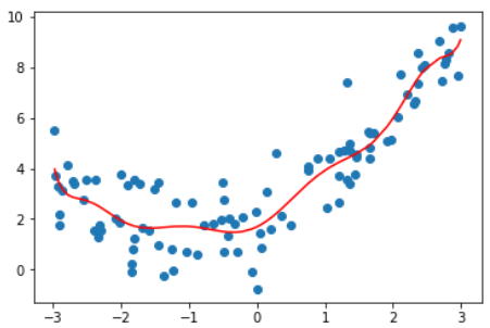 |
| 100 | 0.6880004678712686 | 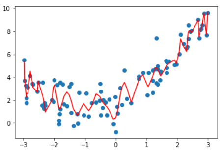 |
这张图不是特别准确,因为这根曲线只是原有数据点连接出来的结果.
因为有些x点取不到,不能准确描述所有点的y值,
均匀取值x并绘制图像如下
显示这不是我们想要的曲线。
结论:degree越高,对训练样本的拟合越好。
因为当degree足够大,总能找到一根曲线拟合所有的样本点,使得均方误差为0.
虽然拟合结果的均方误差小了,但它并没有真的反应样本点的曲线走势。
它为了拟合所有给定的样本而变得太过复杂,这就是过拟合(over fitting)
相反,如果只是使用一根直线来拟合样本数据,也没有很好的拟合样本的特征。
但它不是太复杂了,而是太简单了,这就是欠拟合(under fitting)
机器学习主要要解决的问题是过拟合问题。
例如这根曲线,虽然这根曲线将样本点拟合得很好,总体误差很低,但如果来了一个新样本,它就不能进行很好的预测了。也就是说,这个模型的泛能力很弱。
泛化能力即由此及彼的能力。
我们训练模型不是为了这些已知的点,而是为也预测。因此模型对训练数据的拟合程度有多好是没有意义的。真正需要的是模型的泛化能力。
解决方法:
训练、测试数据分离。
模型只使用训练数据集获取。测试数据对于模型是全新的数据。
如果模型对于测试数据也有很好的结果,就说模型的泛化能力是很强的。
如果模型对训练数据集的效果好,而对测试数据的效果很差,就说模型的泛化能力很弱,通常是过拟合。
仍使用8-3的数据,degree取不同值时在test数据集上的效果对比
| degree | 在训练数据集上的MSE | 在测试数据集上的MSE | note |
|---|---|---|---|
| 线性 | 3.0750025765636577 | 2.2199965269396573 | |
| 2 | 1.0987392142417856 | 0.80356410562979 | 使用二次模型得到的泛化结果比使用线性模型得到的要好 |
| 10 | 1.050846676376417 | 0.9212930722150768 | 在训练数据集上(8-3)degree取10效果更好,但在测试数据集上degree取10的效果变差了。说明degree取10时它的泛化能力变弱了。 |
| 100 | 0.6880004678712686 | 14075796434.50641 | 在训练数据集上效果最好,在测试数据集上效果极差 |
测试数据集的意义
对于不同的算法,模型复杂度代码不同的意思。
对于多项式回归算法来说,模型复杂度相当于degree,degree越高,模型越复杂。
对于KNN算法来说,K越小,模型越复杂。
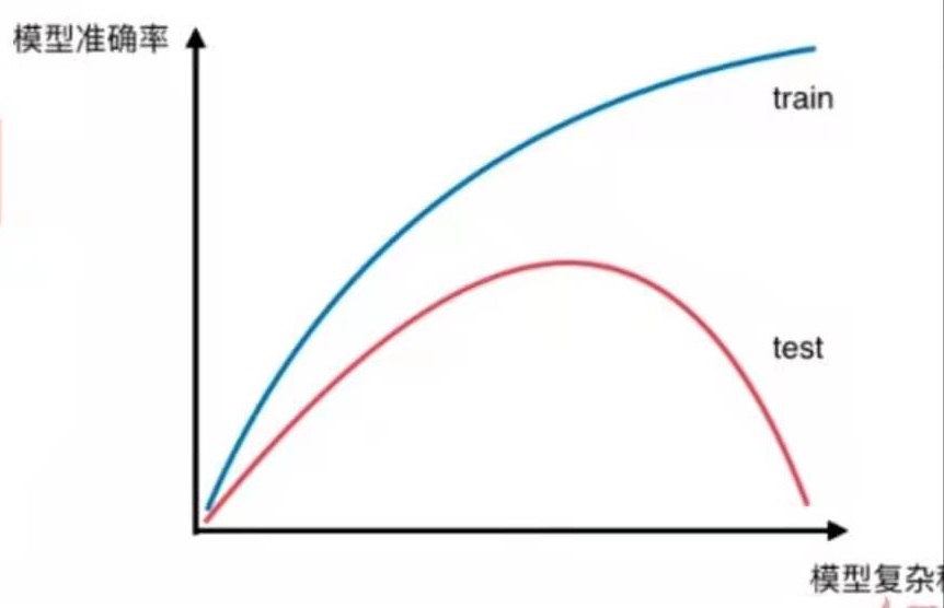
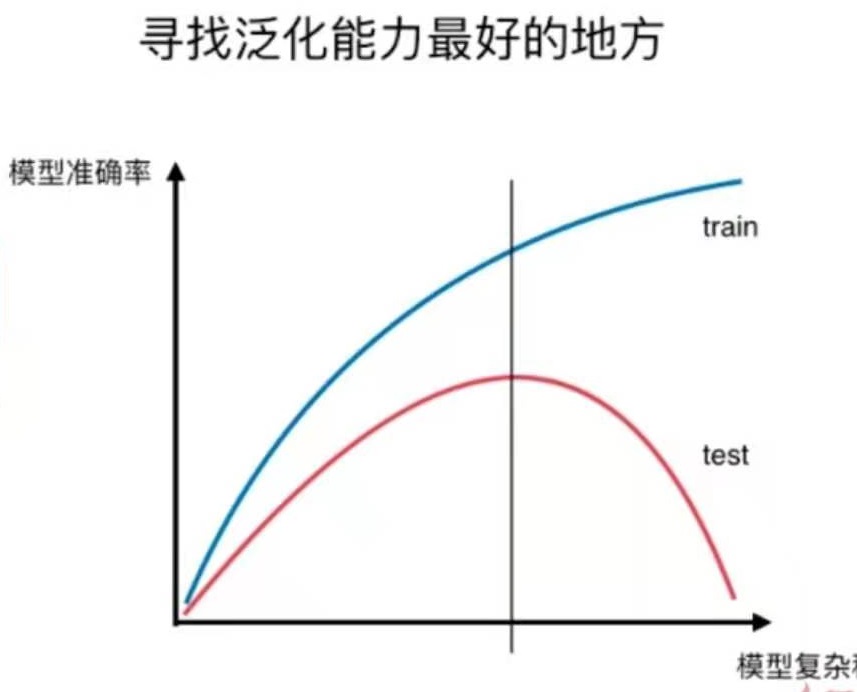
如图所示:
对于训练数据来说,模型越复杂,模型准确率就越高。
对于测试数据来说,模型最简单时,测试数据的准确率会比较低,当模型变复杂时,训练数据的准确率会提升。随着模型越来越复杂,当准确率提升到一定程度时又开始下降。
这就是“欠拟合-合适-过拟合”的过程。
这只是一个示意图,不同模型得到的具体图像不同,但整体上是这样的趋势。
欠拟合 vs 过拟合
欠拟合 underfitting
算法所训练的模型不能完整表述数据关系。
过拟合 overfitting
算法所训练的模型过多地表达了数据间的噪音关系。
这是8-4中提到的模型复杂度曲线。用于说明过拟合和欠拟合。
还有另一种曲线,也可以可视化地表达过拟合与欠拟合的情况,即学习曲线。
学习曲线
随着训练样本的逐渐增多,算法训练出的模型的表现能力。
欠拟合、拟合、过拟合和学习曲线图对比
仍使用8-4中的数据
绘制学习曲线的函数如下:
from sklearn.linear_model import LinearRegression
from sklearn.metrics import mean_squared_error

def plot_learning_curve(algo, X_train, X_test, y_train, y_test):
    train_score = []
    test_score = []
    for i in range(1, len(X_train)+1):
        algo.fit(X_train[:i], y_train[:i])
        y_train_predict = algo.predict(X_train[:i])
        train_score.append(mean_squared_error(y_train[:i], y_train_predict))
        y_test_predict = algo.predict(X_test)
        test_score.append(mean_squared_error(y_test, y_test_predict))

    plt.plot([i for i in range(1, len(X_train)+1)], np.sqrt(train_score), label="train")
    plt.plot([i for i in range(1, len(X_train)+1)], np.sqrt(test_score), label="test")
    plt.legend()
    plt.axis([0, len(X_train)+1, 0, 4])
    plt.show()
线性回归,欠拟合
plot_learning_curve( LinearRegression(), X_train, X_test, y_train, y_test)
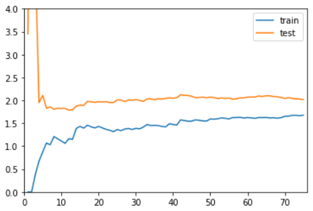
在训练数据集上,误差逐渐升高。
刚开始,误差累积较快,到后面误差累积变慢。
在测试数据集上,刚开始误差很大,逐渐减小,减小到一定程度后达到相对稳定。
最终,训练误差与测试误差趋于大体相同。测试误差略高于训练误差。
2阶多项式回归,拟合
from sklearn.pipeline import Pipeline
from sklearn.preprocessing import PolynomialFeatures
from sklearn.preprocessing import StandardScaler
from sklearn.linear_model import LinearRegression

def PolynomialRegression(degree):
    return Pipeline([
        ("poly", PolynomialFeatures(degree=degree)),
        ("std_scaler", StandardScaler()),
        ("lin_reg", LinearRegression())
    ])

plot_learning_curve( PolynomialRegression(degree=2), X_train, X_test, y_train, y_test)

整体趋势与使用线性回归的图像是一致的。
区别在于,线性回归模型中训练误差和测试误差稳定在1.7左右
而2阶多项式回归模型中训练误差和测试误差稳定在1.0左右
这说明使用2阶多项式回归的结果是比较好的。
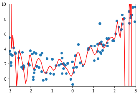
20阶多项式回归,过拟合
plot_learning_curve( PolynomialRegression(degree=20), X_train, X_test, y_train, y_test)
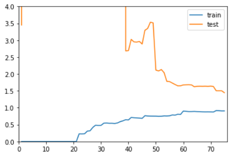
整体趋势仍然是train逐渐上升,test逐渐下降,最终趋于稳定。
在区别是,在train和test都比较稳定时,它们之间的差距是比较大。
这就说明模型虽然在训练数据集上拟合得非常好,但是在测试数据集上误差仍然很大。
这种情况通常就是过拟合。
总结
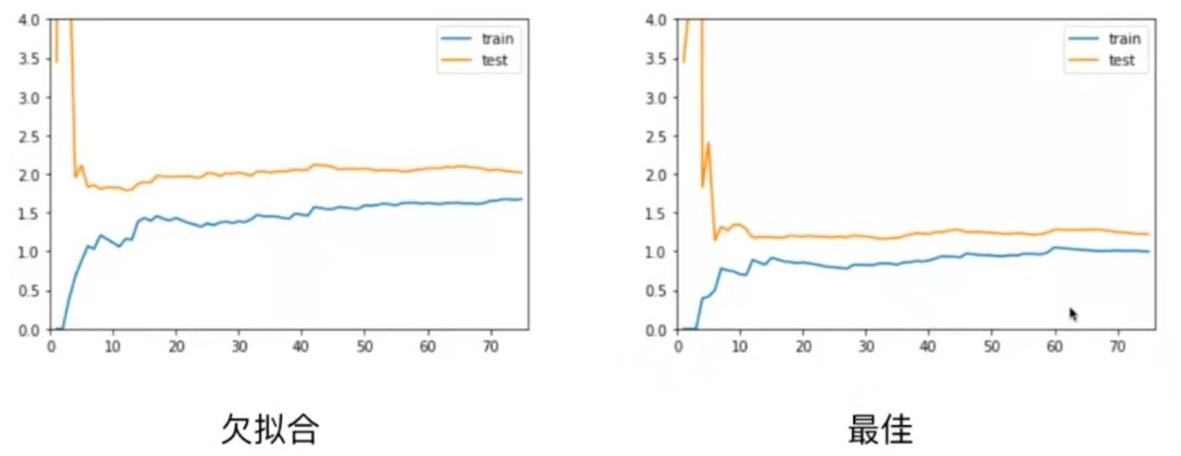 欠拟合情况和最佳情况相比,欠拟合情况train、test曲线趋于稳定的位置比最佳情况的要高一些。这是因为模型选择得不对,所以即使在训练数据集上误差也很大。
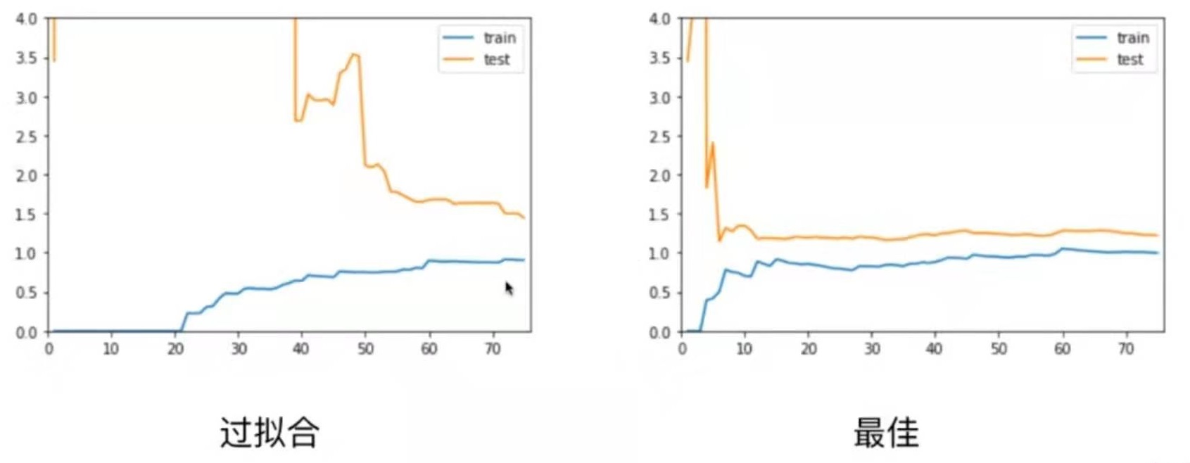 对于过拟合情况,train曲线和最佳情况差不多,但test曲线比较高,并且train与test之间的差距比较大。

问题:发生了过拟合成不自知
解决方法:train test split

训练数据集:训练模型
测试数据集:调整超参数
问题:针对特定测试数据集过拟合?
解决方法:训练 - 验证 - 测试
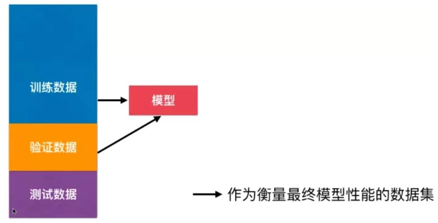
训练数据集:训练模型
验证数据集:调整超参数
测试数据集:不参数模型创建,作为衡量最终模型性能的数据集
问题:随机?一旦验证数据集有异常数据,就会导致模型不准确
解决方法:交叉验证

代码实现
import numpy as np
from sklearn import datasets

digits = datasets.load_digits()
X = digits.data
y = digits.target
测试train_test_split
from sklearn.model_selection import train_test_split
X_train, X_test, y_train, y_test = train_test_split(X, y, test_size=0.4, random_state=666)

from sklearn.neighbors import KNeighborsClassifier

best_score, best_k, best_p = 0,0,0
for k in range(2, 11):
    for p in range(1, 6):
        knn_clf = KNeighborsClassifier(weights="distance", n_neighbors=k, p=p)
        knn_clf.fit(X_train, y_train)
        score = knn_clf.score(X_test, y_test)
        if score > best_score:
            best_score, best_k, best_p = score, k, p

print("best k = ", best_k)
print("best p = ", best_p)
print("best score = ", best_score)
输出结果:
best k = 3
best p = 4
best score = 0.9860917941585535
使用交叉验证
from sklearn.model_selection import cross_val_score

knn_clf = KNeighborsClassifier()
cross_val_score(knn_clf, X_train, y_train)
输出结果:
array([0.98895028, 0.97777778, 0.96629213])
from sklearn.neighbors import KNeighborsClassifier

best_score, best_k, best_p = 0,0,0
for k in range(2, 11):
    for p in range(1, 6):
        knn_clf = KNeighborsClassifier(weights="distance", n_neighbors=k, p=p, cv=3)
        scores = cross_val_score(knn_clf, X_train, y_train)
        score = np.min(scores)
        if score > best_score:
            best_score, best_k, best_p = score, k, p

print("best k = ", best_k)
print("best p = ", best_p)
print("best score = ", best_score)
输出结果:
best k = 2
best p = 2
best score = 0.9823599874006478
train_test_split和交叉验证结果对比:
两种方法得到的best_k和best_p,通常认为使用交叉验证得到参数更可靠。
因为方法一得到的结果很有可能只是过拟合了那一组测试数据。
方法二的分数低于方法一,因为它没有过拟合某一组数据。
best_knn_clf = KNeighborsClassifier(weights="distance", n_neighbors=2, p=2)
best_knn_clf.fit(X_train, y_train)
best_knn_clf.score(X_test, y_test)
输出结果:0.980528511821975
Note:这个算法最终的分类准确度不是上面的0.9823,而是这里的0.9805
回顾网格搜索
from sklearn.model_selection import GridSearchCV

param_grid = [
    {
        'weights':['distance'],
        'n_neighbors': [i for i in range(2, 11)],
        'p': [i for i in range(1, 6)]
    }
]

from sklearn.neighbors import KNeighborsClassifier
knn_clf = KNeighborsClassifier()
grid_search = GridSearchCV(knn_clf, param_grid, cv=3)
grid_search.fit(X_train, y_train)
输入:grid_search.best_score_
输出:0.9823747680890538
输入:grid_search.best_params_
输出:{'n_neighbors': 2, 'p': 2, 'weights': 'distance'}
输入:
best_knn_clf = grid_search.best_estimator_
best_knn_clf.score(X_test, y_test)
输出:0.980528511821975
使用网络搜索与使用交叉验证得到的结果相同。
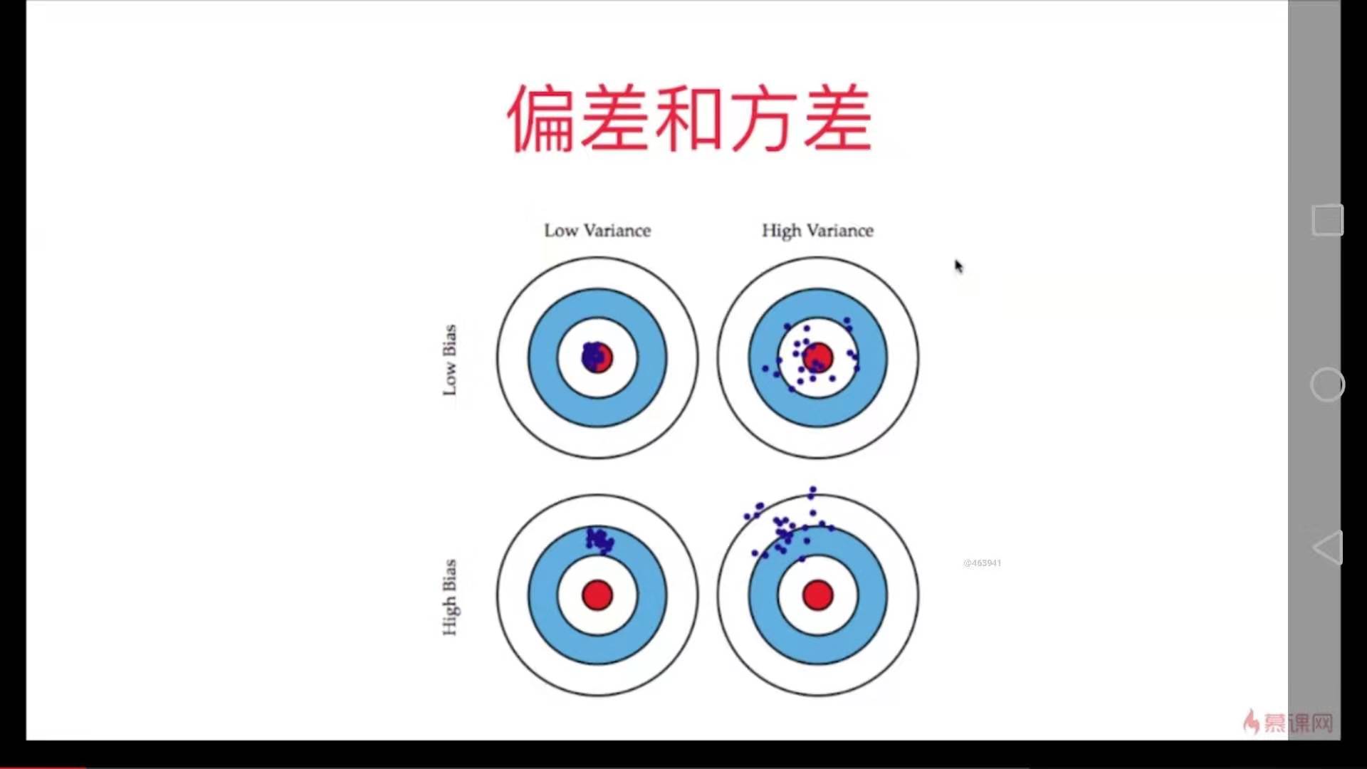
把要解决的问题看作是这个靶盘,训练的模型看作是打出去的枪。
模型的误差 = 偏差 + 方差 + 不可避免的误差
偏差 Bias
导致偏差的原因:
对问题本身的假设不正确。如:非线性数据使用线性回归
欠拟合 underfitting
特征选择不正确
方差 Variance
数据的一点点扰动都会较大地影响模型。
通常原因,使用的模型太复杂,如高阶多项式回归
过拟合 overfitting
偏差和方差
有一些算法天生是高方差的算法。如KNN。
非参数学习算法通常都是高方差算法,因为不对数据做任何假设。
有一些算法天生是高偏差算法。如线性回归。
参数学习算法通常都是高偏差算法。因为对数据有极强的假设性。
大多数算法具有相应的参数,可以调整偏差和方差。 例如KNN中的K、如多项式回归中的degree。
偏差和方差通常是矛盾的。降低偏差,会提高方差。降低方差会提高偏差。
在算法层面上,机器学习的主要挑战来自方差。
解决高方差的通常手段:
- 降低模型复杂度
- 减少数据维度,降噪
- 增加样本数
- 使用验证集
- 模型正则化
模型正则化:限制参数的大小
一个过拟合的例子:
这是8-3中的一个过拟合的例子,把模型的参数打出来如下:

为了尽量地拟合数据,使得线条非常陡峭,数学上表示就是系数非常大
岭回归 Ridge Regularization

Note 1: 正则项是从1累加到n的,theta 0不在里面,因为theta 0代表偏移,不是真正的系数。
Note 2:系数1/2加不加都可以,加了是为了求导方便。
Note 3:a是一个新的超参数,表示目标函数中模型正则化的程度。
代码实现
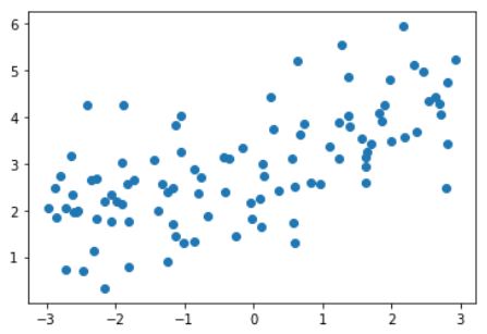
测试数据
import numpy as np
import matplotlib.pyplot as plt

np.random.seed(42)
x = np.random.uniform(-3.0, 3.0, size=100)
X = x.reshape(-1, 1)
y = 0.5 * x + 3 + np.random.normal(0, 1, size=100)

plt.scatter(X, y)
plt.show()
多项式回归,degree = 20
训练模型
from sklearn.pipeline import Pipeline
from sklearn.preprocessing import PolynomialFeatures
from sklearn.preprocessing import StandardScaler
from sklearn.linear_model import LinearRegression

def PolynomialRegression(degree):
    return Pipeline([
        ("poly", PolynomialFeatures(degree=degree)),
        ("std_scaler", StandardScaler()),
        ("lin_reg", LinearRegression())
    ])

from sklearn.model_selection import train_test_split
np.random.seed(666)
X_train, X_test, y_train, y_test = train_test_split(X, y)

from sklearn.metrics import mean_squared_error

poly_reg = PolynomialRegression(degree=20)
poly_reg.fit(X_train, y_train)
绘制模型
def plot_model(model):
    X_plot = np.linspace(-3, 3, 100).reshape(100, 1)
    y_plot = model.predict(X_plot)

    plt.scatter(x, y)
    plt.plot(X_plot[:,0], y_plot, color='r')
    plt.axis([-3, 3, 0, 6])
    plt.show()
训练效果
y_predict = poly_reg.predict(X_test)
mean_squared_error(y_test, y_predict)   # MSE = 167.94010867772357
plot_model(poly_reg)
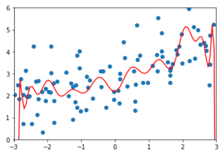
岭回归,degree=20, alpha = 0.0001
训练模型
from sklearn.linear_model import Ridge
from sklearn.pipeline import Pipeline
from sklearn.preprocessing import PolynomialFeatures
from sklearn.preprocessing import StandardScaler
from sklearn.linear_model import LinearRegression

def RidgeRegression(degree, alpha):
    return Pipeline([
        ("poly", PolynomialFeatures(degree=degree)),
        ("std_scaler", StandardScaler()),
        ("ridge_reg", Ridge(alpha=alpha))
    ])

ridge1_reg = RidgeRegression(20, 0.0001)
ridge1_reg.fit(X_train, y_train)
训练效果
y1_predict = ridge1_reg.predict(X_test)
mean_squared_error(y_test, y1_predict)   # MSE = 1.3233492754136291
plot_model(ridge1_reg)
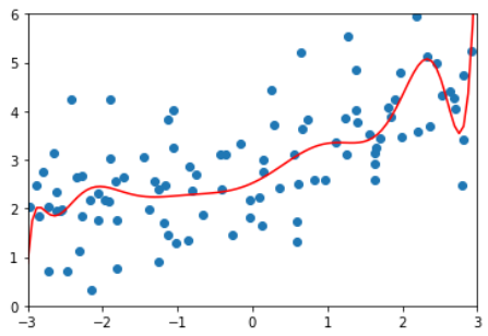
多项式回归及岭回归不同参数的训练结果比较
| MSE | 拟合曲线
--|---|--
多项式回归,degree = 20 | 167.94010867772357 |
岭回归,degree=20, alpha = 0.0001 | 1.3233492754136291 |
岭回归,degree=20, alpha = 1 | 1.1888759304218461 | 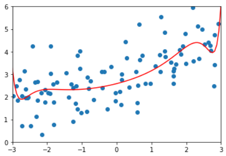 岭回归,degree=20, alpha = 100 | 1.3196456113086197 |
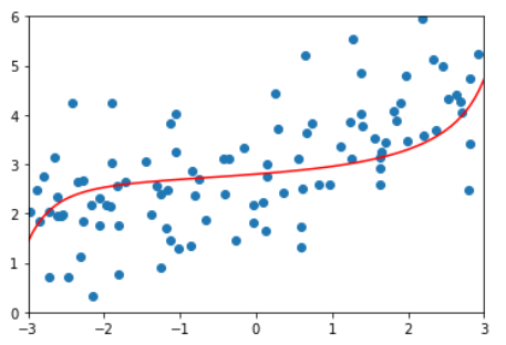
岭回归,degree=20, alpha = 10000000 | 1.840889124848122 | 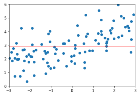
当a非常大时,本质上成了优化正则表达项,即让所有theta=0
LASSO的原理与Ridge相同,只是在怎么表达theta方面选择了一个不同的指标。

LASSO: Least Absolute Shrinkage and Selection Operator Regression
LASSO的效果
使用与8-8相同的测试数据
LASSO回归,degree = 20
训练模型
from sklearn.pipeline import Pipeline
from sklearn.preprocessing import PolynomialFeatures
from sklearn.preprocessing import StandardScaler
from sklearn.linear_model import Lasso

def LassoRegression(degree, alpha):
    return Pipeline([
        ("poly", PolynomialFeatures(degree=degree)),
        ("std_scaler", StandardScaler()),
        ("lasso_reg", Lasso(alpha=alpha))
    ])

from sklearn.model_selection import train_test_split
np.random.seed(666)
X_train, X_test, y_train, y_test = train_test_split(X, y)

from sklearn.metrics import mean_squared_error

lasso1_reg = LassoRegression(degree=20, alpha=0.01)
lasso1_reg.fit(X_train, y_train)

y1_predict = lasso1_reg.predict(X_test)
mean_squared_error(y_test, y1_predict)
MSE = 1.149608084325997
绘制模型
def plot_model(model):
    X_plot = np.linspace(-3, 3, 100).reshape(100, 1)
    y_plot = model.predict(X_plot)

    plt.scatter(x, y)
    plt.plot(X_plot[:,0], y_plot, color='r')
    plt.axis([-3, 3, 0, 6])
    plt.show()

plot_model(lasso1_reg)
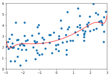
degree=20, 多项式回归、LASSO回归alpha取不同参数的结果对比
| MSE | 拟合曲线
--|---|--
多项式回归,degree = 20 | 167.94010867772357 |
LASSO,degree=20,alpha=0.01 | 1.149608084325997 |
LASSO,degree=20,alpha=0.1 | 1.1213911351818648 | 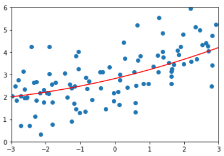
LASSO,degree=20,alpha=1 | 1.8408939659515595 | 
Ridge VS. LASSO
在ridge算法中,随着a的增大,曲线越来越平缓,但它始终是一条曲线。
但在lasso算法中,a取0.1时模型已经接近是直线了。
使用lasso模型得到的更倾向于是一根直线。
直线与曲线的区别在于x的系数theta是否为0。使用lasso中会导致很多特征的系数为0。
lasso趋向于使得一部分theta值变为0,所以可作为特征选择用。
因为如果使用lasso后一部分特征的theta变为0,就代表lasso认为这部分特征是没有用的。
造成ridge和lasso这种区别的原因与它们的导数形式有关。
lasso算法可能会错误地将有用的特征也变为0,从计算准确度角度讲,ridge更准确。
但如果特征数量特别大,使用lasso可以让特征变少。

将类似的思想应用于不同的场景,就成了不同的名词。
其实这些名词背后的数学原理是非常想像的。

在正则化过程中,通常不会使用n>=3的正则项,但理论上是存在的。
L0正则项如下:

求L0正则项是一个NP难问题,所以也不使用。
如果要限制theta的个数,则使用L1代替L0。
弹性网 Elastic Net
超参数r表示两种正则项之间的比例
同时结合了岭回归和lasso回归的优势
在实际应用中通常都先尝试岭回归
但如果特征特别多,岭回归的计算量会特别大,此时优先选择弹性网。
lasso回归则急于将特征化为0,可能会产生一些错误,使得结果偏差较大。
其他
批量梯度下降法 + 随机梯度下降法 = 小批量梯度下降法
岭回归 + lasso回归 = 弹性网
什么是逻辑回归
解决分类问题。
将样本的特征和样本发生的概率联系起来,概率是一个连续的数,因此可以当作回归问题来处理。
对于线性回归,y = f(x)
对于逻辑回归,p = f(x),当p>=0.5,y=1,当p<0.5,y=0
逻辑回归即可以看作是回归算法,也可以看作是分类算法。
通常作为分类算法用,只可以解决二分类问题。
在线性回归中,

y的值域为(-inifinity, inifinity),但概率值的值域[0, 1]
解决方法:
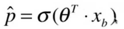
Sigmoid函数
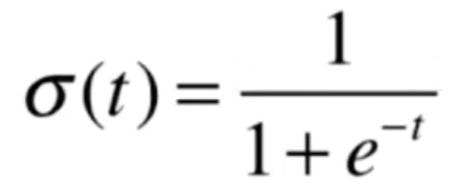
import numpy as np
import matplotlib.pyplot as plt

def sigmoid(t):
    return 1 / (1 + np.exp(-t))

x = np.linspace(-10, 10, 500)
y = sigmoid(x)

plt.plot(x, y)
plt.show()
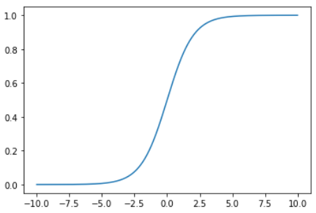
曲线的性质:
左端趋近于但达不到0,右端趋近于但达不到1,即值域(0, 1)
t>0时,p>0.5。t<0时,p<0.5
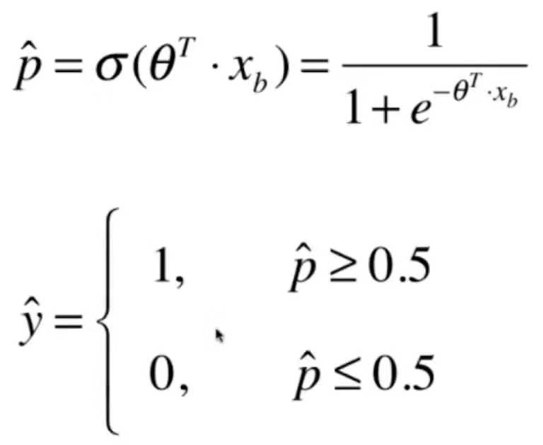
问题:对于给定的样本数据集X,y,我们如何找到参数theta,使得用这样的方式可以最大程度获得样本数据集X对应的分类输出y?
什么是逻辑回归
解决分类问题。
将样本的特征和样本发生的概率联系起来,概率是一个连续的数,因此可以当作回归问题来处理。
对于线性回归,y = f(x)
对于逻辑回归,p = f(x),当p>=0.5,y=1,当p<0.5,y=0
逻辑回归即可以看作是回归算法,也可以看作是分类算法。
通常作为分类算法用,只可以解决二分类问题。
在线性回归中,
y的值域为(-inifinity, inifinity),但概率值的值域[0, 1]
解决方法:
Sigmoid函数
import numpy as np
import matplotlib.pyplot as plt

def sigmoid(t):
    return 1 / (1 + np.exp(-t))

x = np.linspace(-10, 10, 500)
y = sigmoid(x)

plt.plot(x, y)
plt.show()
曲线的性质:
左端趋近于但达不到0,右端趋近于但达不到1,即值域(0, 1)
t>0时,p>0.5。t<0时,p<0.5
问题:对于给定的样本数据集X,y,我们如何找到参数theta,使得用这样的方式可以最大程度获得样本数据集X对应的分类输出y?
问题:对于给定的样本数据集X,y,我们如何找到参数theta,使得用这样的方式可以最大程度获得样本数据集X对应的分类输出y?
cost =
{
如果y = 1,p越小,cost越大
如果y = 0,p越大,cost越大
}
对应的数学公式与几何图像如下:
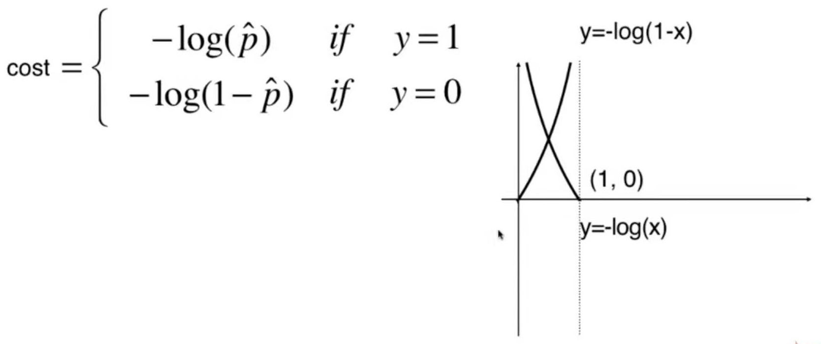
再把以上函数合并成一个函数:
cost = -y*log(p) - (1-y)*log(1-p)
根据所有样本得到的损失函数如下:
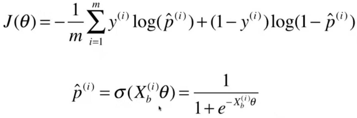
找到一组theta,使得损失函数J(theta)最小。
这个损失函数没有正规方程解,只能使用梯度下降法求解。
这个损失函数是一个凸函数,只有一个最优解。
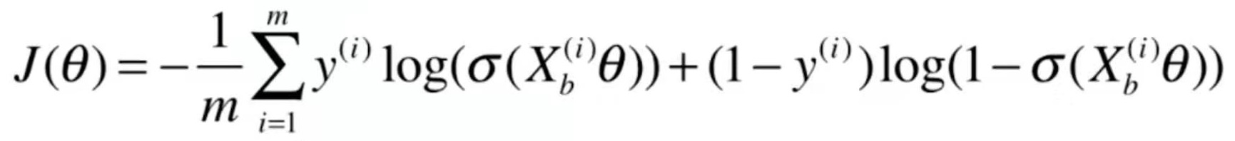
线性回归算法的梯度:
 逻辑回归算法的梯度:
$$
\nabla J(\theta) = \frac{1}{m} \cdot
\begin{Bmatrix}
\sum_{i=1}^m (\hat y^{(i)}-y^{(i)}) \
\sum_{i=1}^m (\hat y^{(i)}-y^{(i)})\cdot X_1^{(i)} \
\sum_{i=1}^m (\hat y^{(i)}-y^{(i)})\cdot X_2^{(i)} \
... \
\sum_{i=1}^m (\hat y^{(i)}-y^{(i)})\cdot X_n^{(i)} \
\end{Bmatrix}
= \frac{1}{m}\cdot X_b^T\cdot (\sigma(X_b\theta)-y)
$$
import numpy as np
from sklearn.metrics import r2_score

class LogisticRegression:

    def __init__(self):
        """初始化Linear Regression模型"""
        self.coef_ = None
        self.interception_ = None
        self._theta = None

    def _sigmoid(self, t):
            return 1. / (1. + np.exp(-t))

    def fit(self, X_train, y_train, eta=0.01, n_iters = 1e4):
        """根据训练数据集X_train, y_train,使用梯度下降法训练Linear Regression模型"""
        assert X_train.shape[0] == y_train.shape[0], "the size of X_train must be equal to the size of y_train"


        def J(theta, X_b, y):
            y_hat = self._sigmoid(X_b.dot(theta))
            try:
                return np.sum(y*np.log(y_hat) + (1-y)*np.log(1-y_hat))
            except:
                return float('inf')

        def dJ(theta, X_b, y):
            return X_b.T.dot(self._sigmoid(X_b.dot(theta))-y) / len(X_b)

        def gradient_descent(X_b, y, initial_theta, eta, n_iters = 1e4, epsilon=1e-8):
            theta = initial_theta
            i_iter = 0
            while i_iter < n_iters:
                gradient = dJ(theta, X_b, y)
                last_theta = theta
                theta = theta - eta * gradient
                if (abs(J(theta, X_b, y) - J(last_theta, X_b, y)) < epsilon):
                    break
                i_iter += 1
            return theta

        X_b = np.hstack([np.ones((len(X_train), 1)), X_train])
        initial_theta = np.zeros(X_b.shape[1])
        self._theta = gradient_descent(X_b, y_train, initial_theta, eta)
        self.interception_ = self._theta[0]
        self.coef_ = self._theta[1:]
        return self

    def predict_proba(self, X_predict):
        """给定待预测数据集X_predict,返回表示X_predict的结果向量"""
        assert self.interception_ is not None and self.coef_ is not None, "must fit before predict"
        assert X_predict.shape[1] == len(self.coef_), "the feature number of X_predict must equal to X_train"

        X_b = np.hstack([np.ones((len(X_predict), 1)), X_predict])
        return self._sigmoid(X_b.dot(self._theta))

    def predict(self, X_predict):
        """给定待预测数据集X_predict,返回表示X_predict的结果向量"""
        assert self.interception_ is not None and self.coef_ is not None, "must fit before predict"
        assert X_predict.shape[1] == len(self.coef_), "the feature number of X_predict must equal to X_train"

        proba = self.predict_proba(X_predict)
        return np.array(proba>=0.5, dtype=int)

    def score(self, X_test, y_test):
        """根据测试数据集X_test, y_test确定当前模型的准确度"""

        y_predict = self.predict(X_test)
        return r2_score(y_test, y_predict)

    def __repr__(self):
        return "LogisticRegression()"
准备数据
import numpy as np
import matplotlib.pyplot as plt
from sklearn import datasets

iris = datasets.load_iris()
X = iris.data
y = iris.target
X = X[y<2, :2]  # 逻辑回归只能解决二分类问题,因此只选取其中两种花的数据
y = y[y<2]

plt.scatter(X[y==0,0],X[y==0,1], color='red')
plt.scatter(X[y==1,0],X[y==1,1], color='blue')
plt.show()
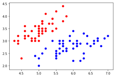
使用逻辑回归
from sklearn.model_selection import train_test_split

X_train, X_test, y_train, y_test = train_test_split(X, y, random_state=666)

log_reg = LogisticRegression()
log_reg.fit(X_train, y_train)

log_reg.score(X_test, y_test)
# 输出:1.0

log_reg.predict_proba(X_test)
# array([0.93292947, 0.98717455, 0.15541379, 0.01786837, 0.03909442,
#        0.01972689, 0.05214631, 0.99683149, 0.98092348, 0.75469962,
#        0.0473811 , 0.00362352, 0.27122595, 0.03909442, 0.84902103,
#        0.80627393, 0.83574223, 0.33477608, 0.06921637, 0.21582553,
#        0.0240109 , 0.1836441 , 0.98092348, 0.98947619, 0.08342411])

y_test
# array([1, 1, 0, 0, 0, 0, 0, 1, 1, 1, 0, 0, 0, 0, 1, 1, 1, 0, 0, 0, 0, 0,
#        1, 1, 0])

log_reg.predict(X_test)
# array([1, 1, 0, 0, 0, 0, 0, 1, 1, 1, 0, 0, 0, 0, 1, 1, 1, 0, 0, 0, 0, 0,
#        1, 1, 0])
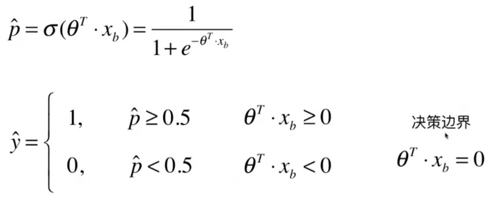 如果X有两个特征,则
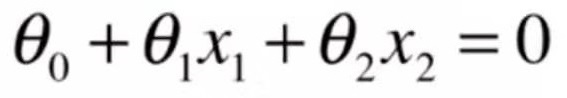 决策边界为:
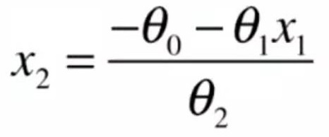
绘制决策边界
仍使用9-4中的例子
def x2(x1):
    return (-log_reg.coef_[0] * x1 - log_reg.interception_) / log_reg.coef_[1]

x1_plot = np.linspace(4, 8, 1000)
x2_plot = x2(x1_plot)

plt.plot(x1_plot, x2_plot)
plt.scatter(X[y==0,0],X[y==0,1], color='red')
plt.scatter(X[y==1,0],X[y==1,1], color='blue')
plt.show()

不规则的决策边界的绘制方法

def plot_decision_boundary(model, axis):
    x0, x1 = np.meshgrid(
        np.linspace(axis[0], axis[1], int((axis[1]-axis[0])*100)).reshape(-1,1),
        np.linspace(axis[2], axis[3], int((axis[3]-axis[2])*100)).reshape(-1,1)
    )
    X_new = np.c_[x0.ravel(), x1.ravel()]

    y_predict = model.predict(X_new)
    zz = y_predict.reshape(x0.shape)

    from matplotlib.colors import ListedColormap
    custom_cmap = ListedColormap(['#EF9A9A','#FFF59D','#90CAF9'])

    plt.contourf(x0, x1, zz, cmap=custom_cmap)
逻辑回归的决策边界
plot_decision_boundary(log_reg, axis=[4,7.5,1.5,4.5])
plt.scatter(X[y==0,0],X[y==0,1], color='red')
plt.scatter(X[y==1,0],X[y==1,1], color='blue')
plt.show()
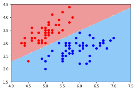
KNN分类算法的决策边界
from sklearn.neighbors import KNeighborsClassifier

knn_clf = KNeighborsClassifier()
knn_clf.fit(X_train, y_train)

plot_decision_boundary(knn_clf, axis=[4,7.5,1.5,4.5])
plt.scatter(X[y==0,0],X[y==0,1], color='red')
plt.scatter(X[y==1,0],X[y==1,1], color='blue')
plt.show()

用KNN对三种iris进行分类的决策边界
knn_clf_all = KNeighborsClassifier()
knn_clf_all.fit(iris.data[:,:2], iris.target)

plot_decision_boundary(knn_clf_all, axis=[4,8,1.5,4.5])
plt.scatter(iris.data[iris.target==0,0],iris.data[iris.target==0,1], color='red')
plt.scatter(iris.data[iris.target==1,0],iris.data[iris.target==1,1], color='blue')
plt.scatter(iris.data[iris.target==2,0],iris.data[iris.target==2,1], color='green')
plt.show()

上图中,黄色与蓝色之间的边界存在过拟合
用KNN对三种iris进行分类的决策边界, K=50
knn_clf_all = KNeighborsClassifier(n_neighbors=50)
knn_clf_all.fit(iris.data[:,:2], iris.target)

plot_decision_boundary(knn_clf_all, axis=[4,8,1.5,4.5])
plt.scatter(iris.data[iris.target==0,0],iris.data[iris.target==0,1], color='red')
plt.scatter(iris.data[iris.target==1,0],iris.data[iris.target==1,1], color='blue')
plt.scatter(iris.data[iris.target==2,0],iris.data[iris.target==2,1], color='green')
plt.show()
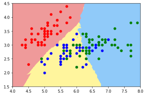
KNN模型中,k值越大,模型越简单
直线这种分类方式太简单,如图这种情况,不可能使用一根直线把样本分成两部分,但它可以使用一个圆形来分割。
因此,对于图中这个样本来说,决策边界应该是x1^2 + x2^2 -r^2 = 0。怎样得到这样的决策边界呢?
解决方法:引入多项式项。

准备数据
import numpy as np
import matplotlib.pyplot as plt

np.random.seed(666)
X = np.random.normal(0, 1, size=(200,2))
y = np.array(X[:,0]**2 + X[:,1]**2 < 1.5, dtype='int')

plt.scatter(X[y==0,0],X[y==0,1])
plt.scatter(X[y==1,0],X[y==1,1])
plt.show()
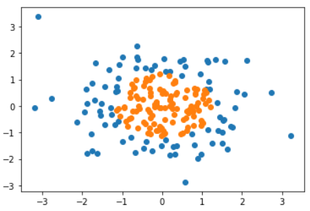
使用逻辑回归
log_reg = LogisticRegression()   # 使用9-4中实现的LogisticRegression类
log_reg.fit(X, y)

log_reg.score(X, y)   # score = 0.605
plot_decision_boundary(log_reg, axis=[-4,4,-4,4])   # 使用9-5中的绘制决策边界的函数
plt.scatter(X[y==0,0],X[y==0,1])
plt.scatter(X[y==1,0],X[y==1,1])
plt.show()
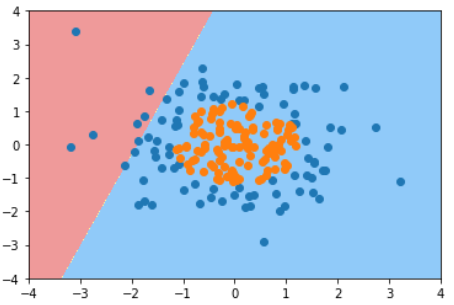
逻辑回归 + 多项式
from sklearn.pipeline import Pipeline
from sklearn.preprocessing import PolynomialFeatures
from sklearn.preprocessing import StandardScaler

def PolynomialLogisticRegression(degree):
    return Pipeline([
        ('poly', PolynomialFeatures(degree=degree)),
        ('std_scaler', StandardScaler()),
        ('log_reg', LogisticRegression())   # 遵循sklearn标准构建的类可以无缝结合到管道中
    ])

poly_log_reg = PolynomialLogisticRegression(degree=2)
poly_log_reg.fit(X, y)
plot_decision_boundary(poly_log_reg, axis=[-4,4,-4,4])
plt.scatter(X[y==0,0],X[y==0,1])
plt.scatter(X[y==1,0],X[y==1,1])
plt.show()
degree取2时的决策边界:
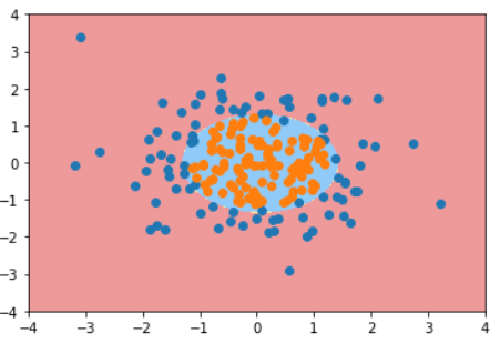
degree取20时的决策边界:
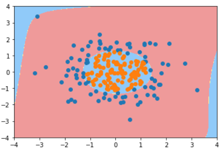
Note 1:代码中的LogisticRegression是在9-4中自己实现的类。只要是遵循sklearn标准构建的类可以无缝结合到管道中。
Note 2:逻辑回归中如果使用了多项式,也可以使用与多项式回归相同的正则表达式来约束过拟合的情况。
在逻辑回归中引入了多项式,模型就会变得复杂,容易出现过拟合。
解决过拟合一个常规的手段就是在模型中添加正则化。
新的目标函数可以是:
J(theta) + a * L2或J(theta) + a * L1,其中a用于表示正则项的重要程度。
但在逻辑回归中,通常这样正则化:
C * J(theata) + L1或C * J(theata) + L2
准备数据
import numpy as np
import matplotlib.pyplot as plt

np.random.seed(666)
X = np.random.normal(0, 1, size=(200,2))
y = np.array(X[:,0]**2 + X[:,1]<1.5, dtype='int')
for _ in range(20):
    y[np.random.randint(200)] = 1

plt.scatter(X[y==0,0],X[y==0,1])
plt.scatter(X[y==1,0],X[y==1,1])
plt.show()
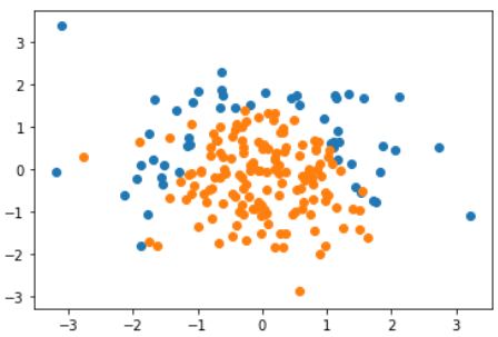
使用逻辑回归
from sklearn.linear_model import LogisticRegression

log_reg = LogisticRegression()
log_reg.fit(X_train, y_train)

log_reg.score(X_train, y_train)   # 0.79333
log_reg.score(X_test, y_test)     # 0.86

plot_decision_boundary(log_reg, [-4, 4, -4, 4])   # 使用8-6中的边界绘制算法
plt.scatter(X[y==0,0],X[y==0,1])
plt.scatter(X[y==1,0],X[y==1,1])
plt.show()
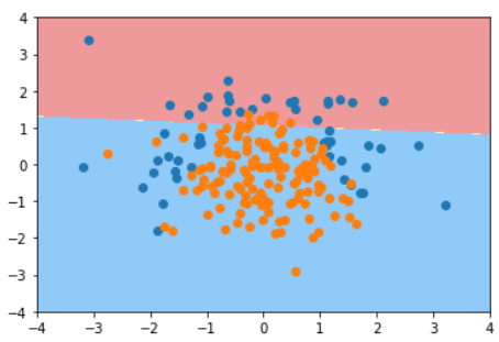
逻辑回归 + 多项式
from sklearn.pipeline import Pipeline
from sklearn.preprocessing import PolynomialFeatures
from sklearn.preprocessing import StandardScaler
from sklearn.linear_model import LogisticRegression

def PolynomialLogisticRegression(degree, C=1.0, penalty='l2'):
    return Pipeline([
        ('poly', PolynomialFeatures(degree=degree)),
        ('std_scaler', StandardScaler()),
        ('log_reg', LogisticRegression(C=C, penalty=penalty))   # 遵循sklearn标准构建的类可以无缝结合到管道中
    ])
使用不同阶数和正则化算法和C值的结果对比
| poly_log_reg.score(X_train, y_train) | poly_log_reg.score(X_test, y_test) | plot_decision_boundary(poly_log_reg, [-4, 4, -4, 4])
--|---|---|--
degree=2 | 0.9133333333333333 | 0.94 | 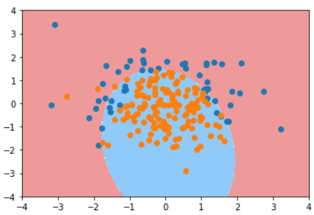
degree=20 | 0.94 | 0.92 | 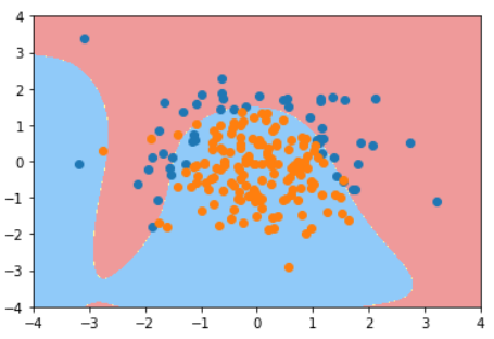
degree=20, C=0.1 | 0.8533333333333334 | 0.92(泛化能力没有降低) | 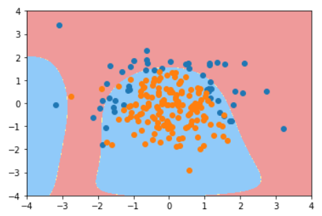
degree=20, C=0.1, penalty='l1' | 0.8266666666666667 | 0.9 | 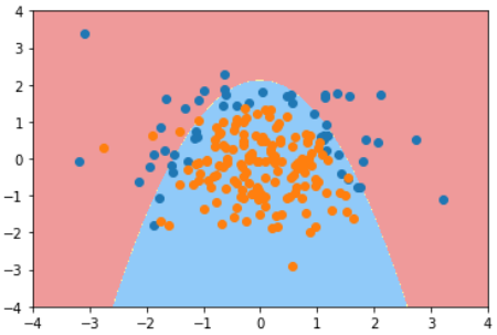
逻辑回归只能解决二分类问题
解决方法:OvR(One vs Rest), OvO(One vs One)
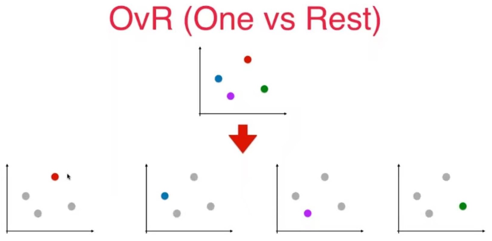
N个类型就进行N次分类,选择得分最高的
对于逻辑回归,这里的分类是指分类的概率
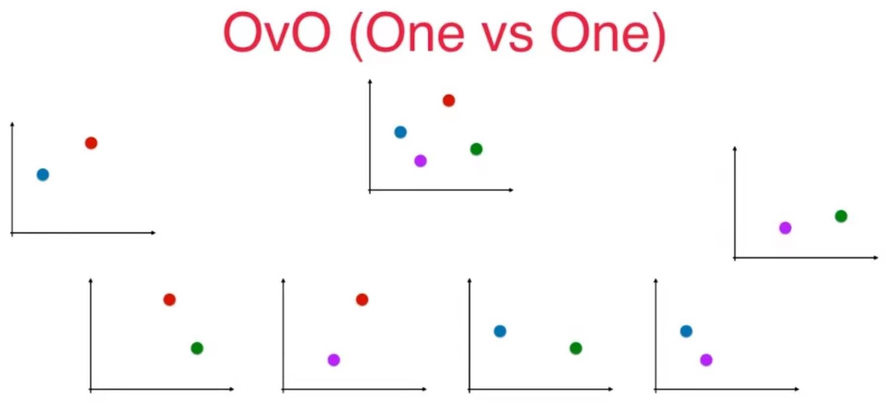
N个类别就进行C(N,2)次分类,选择赢数最多的分类
OvO算法耗时更多,但分类更准确。
使用LogisticRegression提供的ovr和ovo
加载数据
import numpy as np
import matplotlib.pyplot as plt
from sklearn import datasets

iris = datasets.load_iris()
X = iris.data[:, :2]
y = iris.target

from sklearn.model_selection import train_test_split
X_train, X_test, y_train, y_test = train_test_split(X, y, random_state=666)
OvR
from sklearn.linear_model import LogisticRegression
log_reg = LogisticRegression(multi_class='ovr')
log_reg.fit(X_train, y_train)
log_reg.score(X_test, y_test)  # 0.6578947368421053
plot_decision_boundary(log_reg, axis=[4,8,1.5,4.5])   # 见9-5
plt.scatter(iris.data[iris.target==0,0],iris.data[iris.target==0,1], color='red')
plt.scatter(iris.data[iris.target==1,0],iris.data[iris.target==1,1], color='blue')
plt.scatter(iris.data[iris.target==2,0],iris.data[iris.target==2,1], color='green')
plt.show()
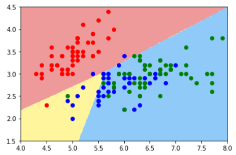
OvO
from sklearn.linear_model import LogisticRegression
log_reg2 = LogisticRegression(multi_class='multinomial', solver='newton-cg')
log_reg2.fit(X_train, y_train)
log_reg2.score(X_test, y_test)   # 0.7894736842105263
plot_decision_boundary(log_reg2, axis=[4,8,1.5,4.5])
plt.scatter(iris.data[iris.target==0,0],iris.data[iris.target==0,1], color='red')
plt.scatter(iris.data[iris.target==1,0],iris.data[iris.target==1,1], color='blue')
plt.scatter(iris.data[iris.target==2,0],iris.data[iris.target==2,1], color='green')
plt.show()
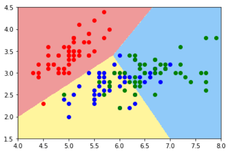
使用所有数据
X = iris.data
y = iris.target
from sklearn.model_selection import train_test_split
X_train, X_test, y_train, y_test = train_test_split(X, y, random_state=666)

from sklearn.linear_model import LogisticRegression
log_reg = LogisticRegression(multi_class='ovr')
log_reg.fit(X_train, y_train)
log_reg.score(X_test, y_test)    # 0.9473684210526315

log_reg2 = LogisticRegression(multi_class='multinomial', solver='newton-cg')
log_reg2.fit(X_train, y_train)
log_reg2.score(X_test, y_test)   # 1.0
使用scikit-learn中的OvR和OvO,能把所有二分类算法转换成多分类算法
log_reg = LogisticRegression()

from sklearn.multiclass import OneVsRestClassifier
ovr = OneVsRestClassifier(log_reg)
ovr.fit(X_train, y_train)
ovr.score(X_test, y_test)   # 0.9473684210526315

from sklearn.multiclass import OneVsOneClassifier
log_reg = LogisticRegression()
ovo = OneVsOneClassifier(log_reg)
ovo.fit(X_train, y_train)
ovo.score(X_test, y_test)   # 1.0
假设有一个算法,其预测某种癌症的准确率为99.9%。这个算法好吗?
999%的准确率看上去很高,但是如果这种癌症本身的发病率只有0.1%,即使不训练模型而直接预测所有人都是健康人,这样的预测的准确率也能达到99.9%。
更极端的情况,如果这种癌症本身的发病率只有0.01%,这算法预测的准确率还不如直接预测所有人都健康。
对于极度偏斜的数据(skewed data),用准确率评价分类算法好坏有局限性。
解决方法:混淆矩阵
工具:混淆矩阵,以二分类为例
0 - Negative - 阴性, 1 - Positive - 阳性
1是我们关注的部分。
| 预测值:0 | 预测值:1
--|---|--
真实值:0 | 预测Negative正确
TN | 预测Positive错误
FP
真实值:1 | 预测Negative错误
FN | 预测Positive正确
TP
0 - Negative, 1 - Positive
| 预测值:0 | 预测值:1
--|---|--
真实值:0 | 预测Negative正确
TN | 预测Positive错误
FP
真实值:1 | 预测Negative错误
FN | 预测Positive正确
TP
指标:精准率和召回率
精准率 precision = TP / (TP + FP)
召回率 recall = TP / (TP + FN)
在有偏数据中,将1作为真正关注的事件
精准率:预测的关注事件(1)中预测对了的概率
召回率:关注事件发生中被预测到概率
这是网上关于精准率召回率的说明图:
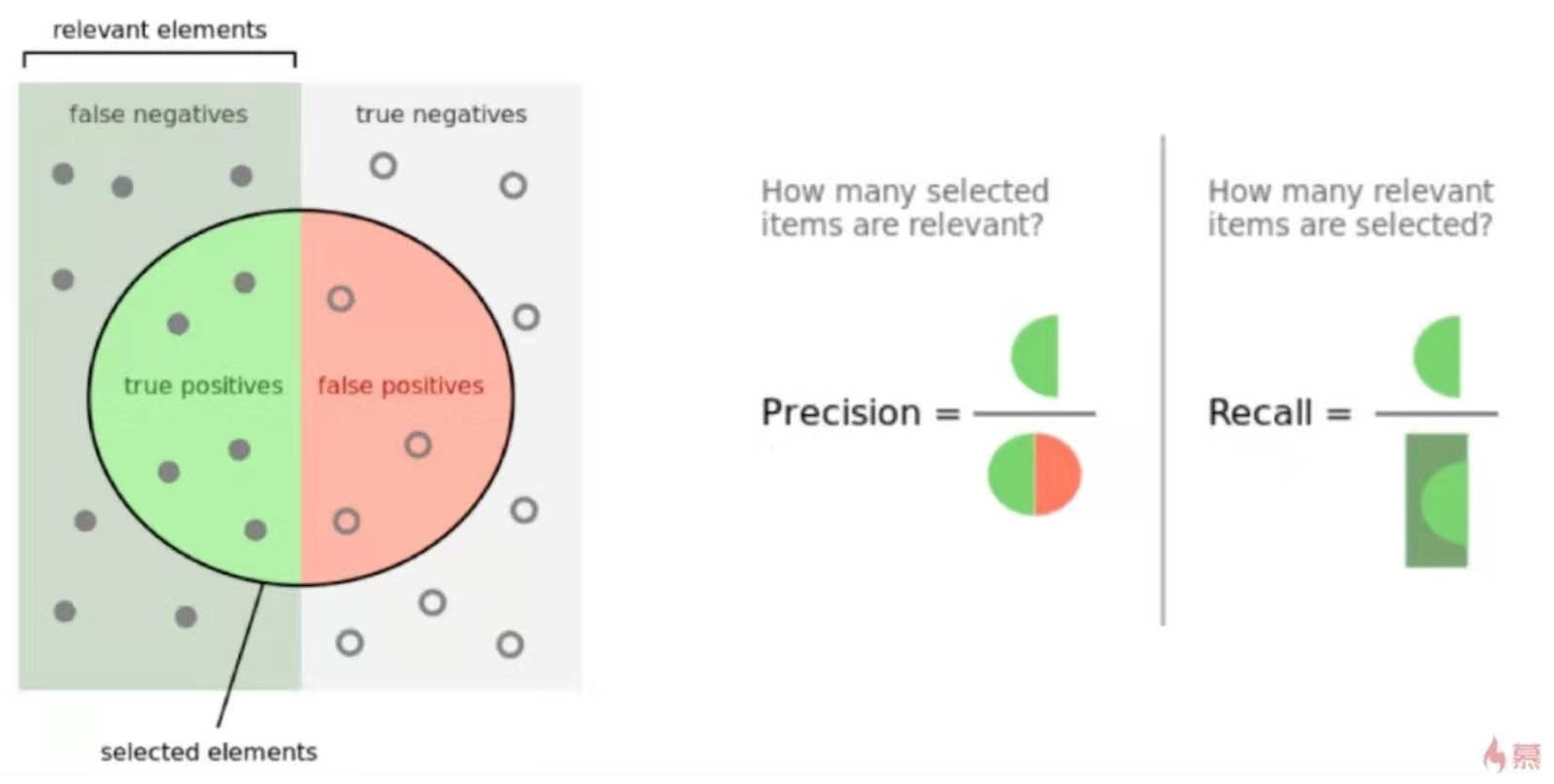
回到9-1中的例子,如果某种癌症的发病率为0.1%,那么预测所有人都健康的模型,虽然准确率达到99.9%。但精准率没有意义,召回率为0,可见这个模型是个无效的模型。
import numpy as np
from sklearn import datasets

digits = datasets.load_digits()
X = digits.data
y = digits.target.copy()

y[digits.target==9] = 1
y[digits.target!=9] = 0    # 产生极度偏斜的数据

from sklearn.model_selection import train_test_split
X_train, X_test, y_train, y_test = train_test_split(X, y, random_state=666)

from sklearn.linear_model import LogisticRegression

log_reg = LogisticRegression()
log_reg.fit(X_train, y_train)
准度度
log_reg.score(X_test, y_test)
输出:0.9755555555555555
混淆矩阵
y_log_predict = log_reg.predict(X_test)

def TN(y_true, y_predict):
    assert len(y_true) == len(y_predict)
    return np.sum((y_true == 0) & (y_predict==0))   # 注意这里是一个‘&’

TN(y_test, y_log_predict)   # 403

def FP(y_true, y_predict):
    assert len(y_true) == len(y_predict)
    return np.sum((y_true == 0) & (y_predict==1))

FP(y_test, y_log_predict)   # 2

def FN(y_true, y_predict):
    assert len(y_true) == len(y_predict)
    return np.sum((y_true == 1) & (y_predict==0))

FN(y_test, y_log_predict)   # 9

def TP(y_true, y_predict):
    assert len(y_true) == len(y_predict)
    return np.sum((y_true == 1) & (y_predict==1))

TP(y_test, y_log_predict)   # 36

def confusion_matrix(y_true, y_predict):
    return np.array([
        [TN(y_true, y_predict), FP(y_true, y_predict)],
        [FN(y_true, y_predict), TP(y_true, y_predict)]
    ])

confusion_matrix(y_test, y_log_predict)
输出结果:
array([[403, 2], [ 9, 36]])
精准率
def precision_score(y_true, y_predict):
    tp = TP(y_true, y_predict)
    fp = FP(y_true, y_predict)
    try:
        return tp / (tp + fp)
    except:   # 处理分母为0的情况
        return 0.0

precision_score(y_test, y_log_predict)
输出结果:0.9473684210526315
召回率
def recall_score(y_true, y_predict):
    tp = TP(y_true, y_predict)
    fn = FN(y_true, y_predict)

    try:
        return tp / (tp + fn)
    except:
        return 0.0

recall_score(y_test, y_log_predict)
输出结果:0.8
scikit-learn中的混淆矩阵、精准率、召回率
from sklearn.metrics import confusion_matrix
confusion_matrix(y_test, y_log_predict)

from sklearn.metrics import precision_score
precision_score(y_test, y_log_predict)

from sklearn.metrics import recall_score
recall_score(y_test, y_log_predict)
对于极度偏斜的数据,使用指标精准率和召回率都优于使用指标分类准确度。
但精准率和召回率是两个指标。如果一个算法的精准率和召回率表现不同,该如何取舍这两个指标?
解决方法1:视具体场景而定。
有时我们注重精准率,比如股票预测,我们希望预测股票为升结果都是准确的(否则可能亏钱),而不在意错过另一些错过的股票上升的机会(错过一些赚钱的机会)。
有时我们注重召回率,比如病人诊断。我们希望得病的人都能识别出来(否则这些人可能会病情恶化),而有一些没得病的人被错误地识别出来没有关系(这些人做进一步检查即可)。
解决方法2:同时关注精准率和召回率,即新指标:F1 score
指标:F1 score
F1 score是precision和recall的调和平均值。
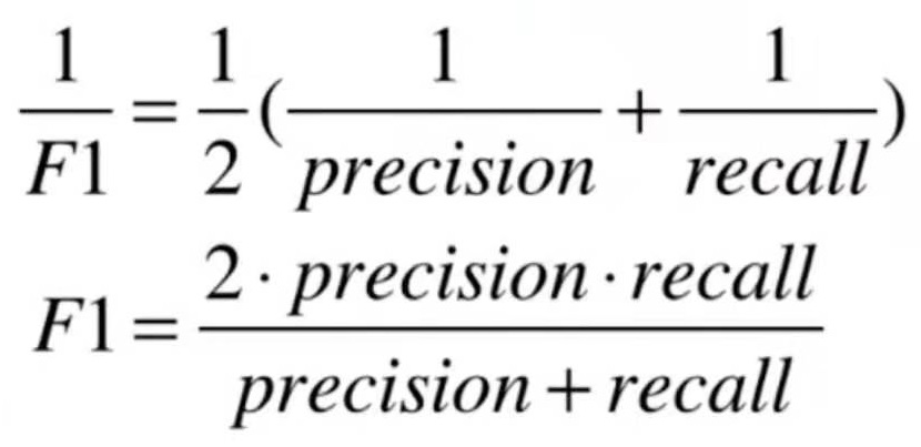
调和平均值的特点:如果precision和recall非常不平衡,则f1 score也是比较低的。只有两者都高,F1 score才会高。
F1 score的取值范围:[0, 1]
自己实现F1 score
import numpy as np
def f1_score(precision, recall):
    try:
        return 2 * precision * recall / (precision + recall)
    except:
        return 0.0
precision和recall取不同的值对f1_score的影响
| precision | racall | f1_score |
|---|---|---|
| 0.5 | 0.5 | 0.5 |
| 0.1 | 0.9 | 0.18 |
| 0.0 | 1.0 | 0 |
对于调和平均值来说,二者有一个分数较低,都会极大的拉低结果。
因此能更好的表征precison和recal这两个指标。
F1 score来评价手写数字的识别效果
使用10-3的测试数据
from sklearn.metrics import f1_score
f1_score(y_test, y_predict)
输出:0.8674698795180723
对有偏数据,指标F1 score优于分类准确度。
我们总是希望精准率和召回率这两个指标都尽可能地高。但事实上精准率和召回率是互相矛盾的,我们只能在其中找到一个平衡。
以逻辑回归为例来说明精准率和召回率之间的矛盾关系,以下是逻辑回归的公式:
$$
\begin{aligned}
\hat p = \sigma(\theta^T \cdot x_b) = \frac{1}{1 + \exp(-\theta^T \cdot x_b)} \
\hat y =
\begin{cases}
1, && \hat p \ge 0.5 && \theta^T \cdot x_b \ge 0 && \text{决策边界} \
0, && \hat p \lt 0.5 && \theta^T \cdot x_b \lt 0 && \theta^T \cdot x_b = 0
\end{cases}
\end{aligned}
$$
在这里决策边界是以0为分界点,如果把0改成一个自定义的threshold,threshold的改变会平移决策边界,从而影响精准率和召回率的结果。
$$
\theta^T \cdot x_b = \text{threshold}
$$
threshold是怎样影响精准率和召回率的
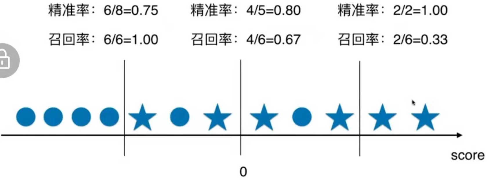
如图,图中的直线代表决策边界,决策边界右边的样本分类为1,决策边界左边的样本分类为0。图中五角星为实际类别为1的样本,0为实际类别为0的样本。
如果以0为分界点,精准率 = 4/5 = 80,召回率 = 4 / 6 = 0.67
分界点往右移,则精准率提升,召回率降低。
分界点往左移,则精准率下降,召回率提升。
用10-4中的Logic Regression对手写数字分类的例子来说明分界点移动对精准率和召回率的影响
回顾10-4的代码
准备数据
import numpy as np
from sklearn import datasets

digits = datasets.load_digits()
X = digits.data
y = digits.target.copy()

y[digits.target==9] = 1
y[digits.target!=9] = 0

from sklearn.model_selection import train_test_split
X_train, X_test, y_train, y_test = train_test_split(X, y, random_state=666)
训练模型
from sklearn.linear_model import LogisticRegression

log_reg = LogisticRegression()
log_reg.fit(X_train, y_train)
模型指标
log_reg.score(X_test, y_test)   #  0.9755555555555555

y_predict = log_reg.predict(X_test)

from sklearn.metrics import confusion_matrix
confusion_matrix(y_test, y_predict)   # array([[403,   2], [  9,  36]], dtype=int64)

from sklearn.metrics import precision_score
precision_score(y_test, y_predict)   # 0.9473684210526315

from sklearn.metrics import recall_score
recall_score(y_test, y_predict)   # 0.8

from sklearn.metrics import f1_score
f1_score(y_test, y_predict)   # 0.8674698795180723
移动Logic Regression的分界点
分析Logic Regression当前使用的分界点
上文中提到,通过调整threshold来移动决策边界,但sklearn并没有直接提供这样的接口。自带predict函数都是以0作为threshold的。
但sklearn提供了决策函数,把X_test传进去,得到的是每个样本的score值。
predict函数就是根据样本的score值来判断它的分类结果。
log_reg.decision_function(X_test)
部分输出截图:

例如前10个样本的score值是这样的,那么它们的predict结果都应该为0
log_reg.decision_function(X_test)[:10]与log_reg.predict(X_test)[:10]对比:
array([-22.05700117, -33.02940957, -16.21334087, -80.3791447 ,
-48.25125396, -24.54005629, -44.39168773, -25.04292757,
-0.97829292, -19.7174399 ])
array([0, 0, 0, 0, 0, 0, 0, 0, 0, 0])
所以可以基于decision_function来移动决策边界。
decision_scores = log_reg.decision_function(X_test)
np.min(decision_scores)   # -85.68608522646575
np.max(decision_scores)   # 19.8895858799022
移动threshold: 0->5
y_predict_2 = np.array(decision_scores >= 5, dtype='int')
confusion_matrix(y_test, y_predict_2)   # array([[404,   1], [ 21,  24]], dtype=int64)
precision_score(y_test, y_predict_2)   # 0.96
recall_score(y_test, y_predict_2)   # 0.5333333333333333
不同分界点的指标对比
| threshold | confusion_matrix | precision_score | recall_score |
|---|---|---|---|
| decision_scores >= 0(default) | array([[403, 2], [ 9, 36]], dtype=int64) | 0.9473684210526315 | 0.8 |
| decision_scores >= 5 | array([[404, 1], [ 21, 24]], dtype=int64) | 0.96 | 0.5333333333333333 |
| decision_scores >= -5 | array([[390, 15], [ 5, 40]], dtype=int64) | 0.7272727272727273 | 0.8888888888888888 |
先回顾一下上一节课的代码
import numpy as np
from sklearn import datasets

digits = datasets.load_digits()
X = digits.data
y = digits.target.copy()

y[digits.target==9] = 1
y[digits.target!=9] = 0

from sklearn.model_selection import train_test_split
X_train, X_test, y_train, y_test = train_test_split(X, y, random_state=666)

from sklearn.linear_model import LogisticRegression

log_reg = LogisticRegression()
log_reg.fit(X_train, y_train)
log_reg.score(X_test, y_test)
输出:0.9755555555555555
skleran的Logical Regression中,通过discision score和threshold来判断分类结果。
默认情况下threshold = 0。
调整threshold值,精准率和召回率就会相应的变化。
这一节通过可视化的方式表现threshold和精准率、召回率之间的关系。
精准率和召回率的变化曲线
decision_scores = log_reg.decision_function(X_test)

from sklearn.metrics import precision_score
from sklearn.metrics import recall_score
import matplotlib.pyplot as plt

precision_scores = []
recall_scores = []

thresholds = np.arange(np.min(decision_scores), np.max(decision_scores), step=0.1)
for threshold in thresholds:
    y_predict = np.array(decision_scores >= threshold, dtype='int')
    precision_scores.append(precision_score(y_test, y_predict))
    recall_scores.append(recall_score(y_test, y_predict))

plt.plot(thresholds, precision_scores)
plt.plot(thresholds, recall_scores)
plt.show()
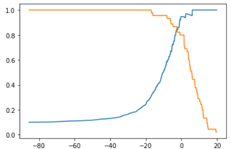
可以根据这张图找到想要的threshold。
绘制precision-recall曲线
plt.plot(precision_scores, recall_scores)
plt.show()

scikit-learn中的precision-recall曲线
from sklearn.metrics import precision_recall_curve

precisions, recalls, thresholds = precision_recall_curve(y_test, decision_scores)
plt.plot(thresholds, precisions[:-1])
plt.plot(thresholds, recalls[:-1])
plt.show()
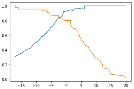
Note 1:precisions.shape = (145,),recalls.shape = (145,),thresholds.shape = (145,),这是因为“the last precision and recall values are 1. and 0. respectively and do not have a corresponding threshold.”
Note 2:sklearn提供的precision-recall曲线自动只寻找了我们最关心的那一部分。
关于precision-recall曲线的理论说明
召回率急剧下降开始的点通常精准率-召回率最好的平衡点。

精准率-召回率曲线整体上是这样的曲线。用不同的算法或相同的算法的不同的超参数都能训练出各自的模型。每种模型都有不同的精准率-召回率曲线。
假如如图是两个模型的精准率-召回率曲线,那么明显可以得出结论外面曲线的模型优于里面曲线的模型。因此PR曲线也可以作为选择模型/超参数的指标。
ROC:Receiver Operation Characteristic Curve
ROC曲线描述TPR和FPR之间的关系。
TPR = recall = TP / (TP + FN) # true positive rate FPR = FP / (FP + TN) # false positive rate
TPR和FPR的关系如图:

TPR和FRP呈现相一致的趋势
代码
回顾前面学过的代码
def TN(y_true, y_predict):
    assert len(y_true) == len(y_predict)
    return np.sum((y_true == 0) & (y_predict==0))   # 注意这里是一个‘&’

def FP(y_true, y_predict):
    assert len(y_true) == len(y_predict)
    return np.sum((y_true == 0) & (y_predict==1))

def FN(y_true, y_predict):
    assert len(y_true) == len(y_predict)
    return np.sum((y_true == 1) & (y_predict==0))

def TP(y_true, y_predict):
    assert len(y_true) == len(y_predict)
    return np.sum((y_true == 1) & (y_predict==1))

def confusion_matrix(y_true, y_predict):
    return np.array([
        [TN(y_true, y_predict), FP(y_true, y_predict)],
        [FN(y_true, y_predict), TP(y_true, y_predict)]
    ])

def precision_score(y_true, y_predict):
    tp = TP(y_true, y_predict)
    fp = FP(y_true, y_predict)
    try:
        return tp / (tp + fp)
    except:   # 处理分母为0的情况
        return 0.0

def recall_score(y_true, y_predict):
    tp = TP(y_true, y_predict)
    fn = FN(y_true, y_predict)

    try:
        return tp / (tp + fn)
    except:
        return 0.0
TPR和FPR
def TPR(y_true, y_predict):
    tp = TP(y_true, y_predict)
    fn = FN(y_true, y_predict)

    try:
        return tp / (tp + fn)
    except:
        return 0.0

def FPR(y_true, y_predict):
    fp = FP(y_true, y_predict)
    tn = TN(y_true, y_predict)

    try:
        return fp / (fp + tn)
    except:
        return 0.0
加载测试数据
import numpy as np
from sklearn import datasets

digits = datasets.load_digits()
X = digits.data
y = digits.target.copy()

y[digits.target==9] = 1
y[digits.target!=9] = 0

from sklearn.model_selection import train_test_split
X_train, X_test, y_train, y_test = train_test_split(X, y, random_state=666)

from sklearn.linear_model import LogisticRegression

log_reg = LogisticRegression()
log_reg.fit(X_train, y_train)
绘制TFP和FRP的曲线,即ROC
decision_scores = log_reg.decision_function(X_test)
import matplotlib.pyplot as plt

fprs = []
tprs = []

thresholds = np.arange(np.min(decision_scores), np.max(decision_scores), step=0.1)
for threshold in thresholds:
    y_predict = np.array(decision_scores >= threshold, dtype='int')
    fprs.append(FPR(y_test, y_predict))
    tprs.append(TPR(y_test, y_predict))

plt.plot(fprs, tprs)
plt.show()

sklearn中的ROC曲线
from sklearn.metrics import roc_curve

fprs, tprs, thresholds = roc_curve(y_test, decision_scores)
plt.plot(fprs, tprs)
plt.show()
我们通常关注这条曲线下面的面积。面积越大,说明分类的效果越好。
ROC score
ROC score代码曲线下面的面积。
auc = area under curl
from sklearn.metrics import roc_auc_score
roc_auc_score(y_test, decision_scores)
输出:0.9830452674897119
总结
对于有偏数据,观察它的精准率和召回率是非常有必要的。
但是ROC曲线对有偏数据并不敏感,它主要用于比较两个模型的孰优孰劣。
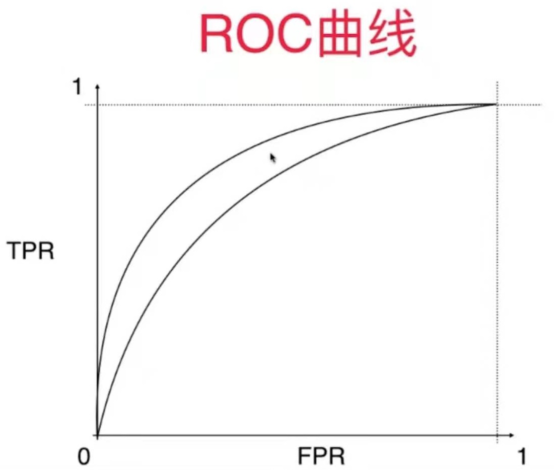
如果两根曲线分别代码两个模型的ROC曲线,在这种情况下我们会选择外面那根曲线对应模型。
前面小节就针对二分类问题的,这一节把这些指标扩展到多分类问题。
加载手写数据集
import numpy as np
from sklearn import datasets

digits = datasets.load_digits()
X = digits.data
y = digits.target

from sklearn.model_selection import train_test_split
X_train, X_test, y_train, y_test = train_test_split(X, y, test_size=0.8,random_state=666)
使用逻辑回归训练模型
from sklearn.linear_model import LogisticRegression
log_reg = LogisticRegression()
log_reg.fit(X_train, y_train)
log_reg.score(X_test, y_test)
输出:0.93115438108484
计算精准率
y_predict = log_reg.predict(X_test)
from sklearn.metrics import precision_score
precision_score(y_test, y_predict)
会报错,因为默认只能为二分类问题计算精准率
解决方法:

from sklearn.metrics import precision_score
precision_score(y_test, y_predict, average='micro')
输出:0.93115438108484
计算混淆矩阵并可视化
计算混淆矩阵
混淆矩阵天然支持多分类问题。
from sklearn.metrics import confusion_matrix
confusion_matrix(y_test, y_predict)
输出:
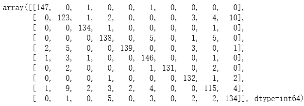
第i行第j列代表真值为i而预测值为j的样本数量。
对角线位置是预测正确的位置。
把矩阵可视化,可以直观地看到犯错误比较多的地方。
可视化
import matplotlib.pyplot as plt
cfm = confusion_matrix(y_test, y_predict)
plt.matshow(cfm, cmap=plt.cm.gray) # 映射成灰度值
plt.show()

越亮的地方代表数值越大。
图中对角线部分太亮,无法观察到我们关心的部分,改进如下:
row_sums = np.sum(cfm, axis=1)
err_matrix = cfm / row_sums
np.fill_diagonal(err_matrix, 0)
err_matrix
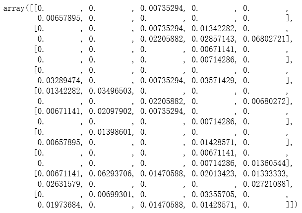
plt.matshow(err_matrix, cmap=plt.cm.gray)
plt.show()
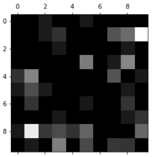 图中越亮的地方表示犯错越多的地方。
针对错误比较多的地方做算法的微调。
Support Vector Machine
既可以解决分类问题,也可以解决回归问题。
支撑向量机的思想
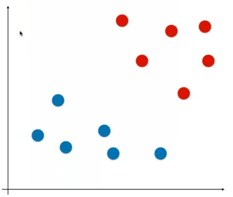
图中是一个样本空间,里面有一些样本点,分成红色和蓝色两类。
逻辑回归是要找到一根决策边界,由决策边界把数据分成两类。但可能存在这样一些数据(下图),可能存在多条决策边界。(不适定问题)
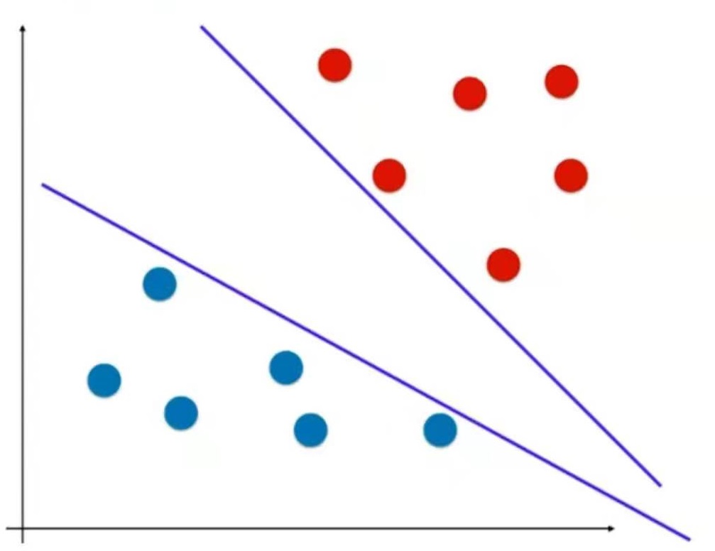
逻辑回归定义了一个损失函数,通过最小化损失函数求出决策边界。
假设逻辑回归算法最后求出的是这样一根直线(下图),它在前面的所给的样本空间中表现很好,但新来这样一个样本,那么很有可能它的分类结果是错误的。

这根决策边界的泛化效果不够好,因为它离红色样本点太近了。那么怎样的决策边界泛化能力比较好呢?
看上去下图这根直线的泛化能力要更好一点。
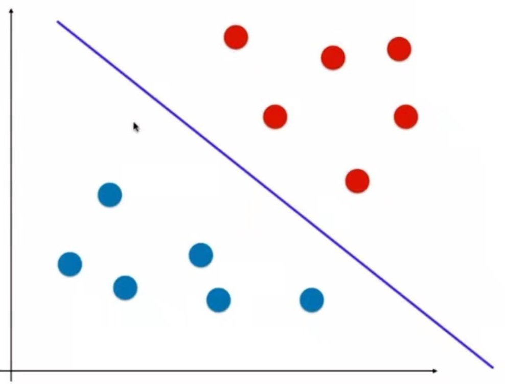
离这根直线最近的点有3个,让这3个点离这根直线的距离尽可能地远。
也就是说,让这个决策边界既离红线尽可能远,也离蓝点尽可能远。于是得到了上图这样的决策边界。
它不仅将训练数据划分开类,还期望它的泛化能力尽可能好。它把对泛化能力的考量直接放到了算法的内部。
把以上的思考用数学方式表达出来就是,让离决策边界最近的三个点,到决策边界的距离应该是一样的并且尽可能地大。
基于这三个点又找两根与决策边界平行的直线。这两根直线定义了一个区域。这个区域中不再有任何点。
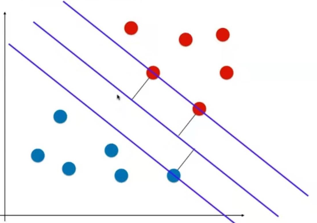
什么是支撑向量机
SVM尝试寻找一个最优的决策边界。
这个决策边界距离两个类别的最近的样本最远。
这三个最近的样本称为支撑向量。
支撑向定义了一个区域,这个区域又定义了最优决策边界。
上下两根直线离决策边界的距离都是d。
上下两根直线之间的距离称为margin.
SVM要最大化margin

SVM只能解决线性可分的问题,即hard Margin SVM.
对hard Margin SVM改进,能解决线性不可分的数据,即soft Margin SVM
Support Vector Machine
既可以解决分类问题,也可以解决回归问题。
支撑向量机的思想
图中是一个样本空间,里面有一些样本点,分成红色和蓝色两类。
逻辑回归是要找到一根决策边界,由决策边界把数据分成两类。但可能存在这样一些数据(下图),可能存在多条决策边界。(不适定问题)
逻辑回归定义了一个损失函数,通过最小化损失函数求出决策边界。
假设逻辑回归算法最后求出的是这样一根直线(下图),它在前面的所给的样本空间中表现很好,但新来这样一个样本,那么很有可能它的分类结果是错误的。
这根决策边界的泛化效果不够好,因为它离红色样本点太近了。那么怎样的决策边界泛化能力比较好呢?
看上去下图这根直线的泛化能力要更好一点。
离这根直线最近的点有3个,让这3个点离这根直线的距离尽可能地远。
也就是说,让这个决策边界既离红线尽可能远,也离蓝点尽可能远。于是得到了上图这样的决策边界。
它不仅将训练数据划分开类,还期望它的泛化能力尽可能好。它把对泛化能力的考量直接放到了算法的内部。
把以上的思考用数学方式表达出来就是,让离决策边界最近的三个点,到决策边界的距离应该是一样的并且尽可能地大。
基于这三个点又找两根与决策边界平行的直线。这两根直线定义了一个区域。这个区域中不再有任何点。
什么是支撑向量机
SVM尝试寻找一个最优的决策边界。
这个决策边界距离两个类别的最近的样本最远。
这三个最近的样本称为支撑向量。
支撑向定义了一个区域,这个区域又定义了最优决策边界。
上下两根直线离决策边界的距离都是d。
上下两根直线之间的距离称为margin.
SVM要最大化margin
SVM只能解决线性可分的问题,即hard Margin SVM.
对hard Margin SVM改进,能解决线性不可分的数据,即soft Margin SVM
SVM要最大化margin,即图中两根直线之间的距离
用数学语言来表达: margin = 2 * d,最大化d就是最大化margin
点x到直线$$w^T * x + b = 0$$的距离为:
$$
distance = \frac{|w^T+b|}{||w||} \
||w|| = \sqrt {w_1^2+w_2^2+\cdots+w_n^2}
$$
所有的样本点到决策边界到距离都应该大于d,用于公式表达:

上面这个公式可写成这样的形式:
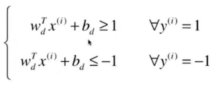
于是可得出margin上下两条直线的方程为:
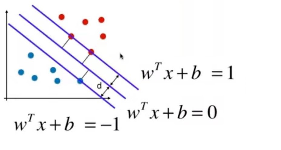
**注意:这里三条直线中的已经不是原来的$$w^T$$和b了,$$w_b^T=w^T/(||w||d), b_d=b/(||w||d)$$
SVM的目标是最大化d,d的公式在上文已经给出。
由于支持向量x一定是在margin的上下边界点上,可以证明对于任意支持向量x,以下四个公式表达的目标的相同的:

结论:
SVM算法演变为有条件的最优化问题,(st:条件)

有条件的最优化问题和没有条件的最优化问题,其求解方法大不相同。
hard Margin:
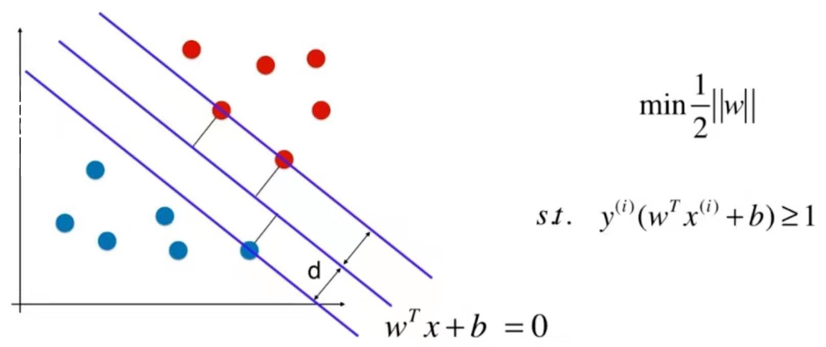
使用这种方法,对下面这张图中的样本,hard SVM会给出这样一根决策边界

hard SVM非常明显地受到一个蓝点的影响,而这个蓝点很有可能是outlier或者是个错误点。
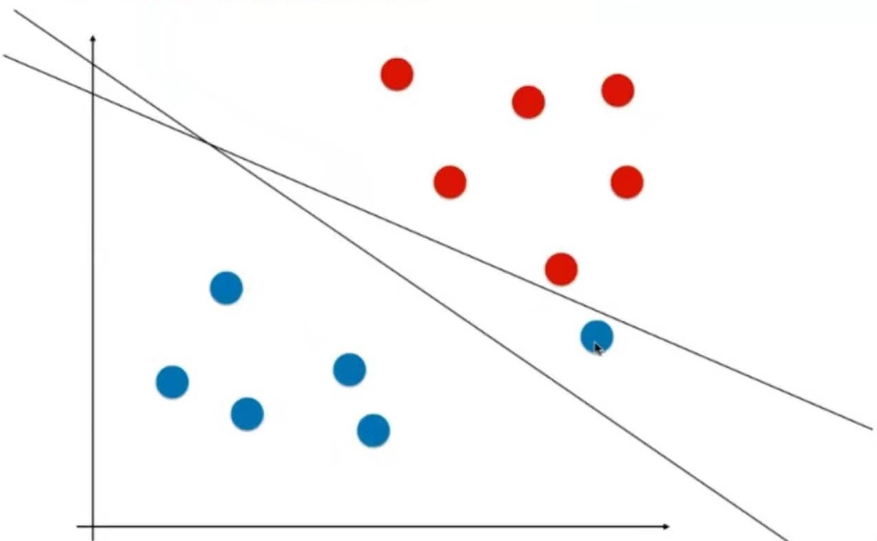
这根决策边界可能是一根更好的决策边界。
而对于下图这样的样本点,线性不可分的情况,hard SVN是无解的。
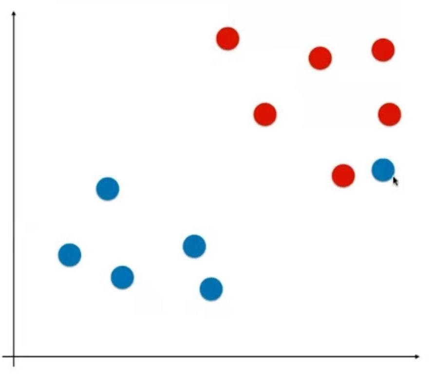
hard SVM需要更好的容错性。
改进:增加一个宽松量
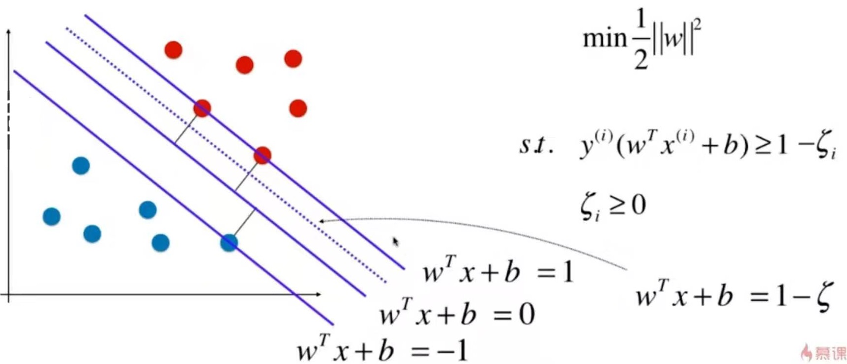
即允许一些点出现在图中虚线和实线之间的位置。
这里的宽松量不是一个定值,它对每一个样本都是不同的。
同时还要最小化所有的宽松量。
目标函数变成了:
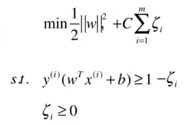
L1正则、L2正则
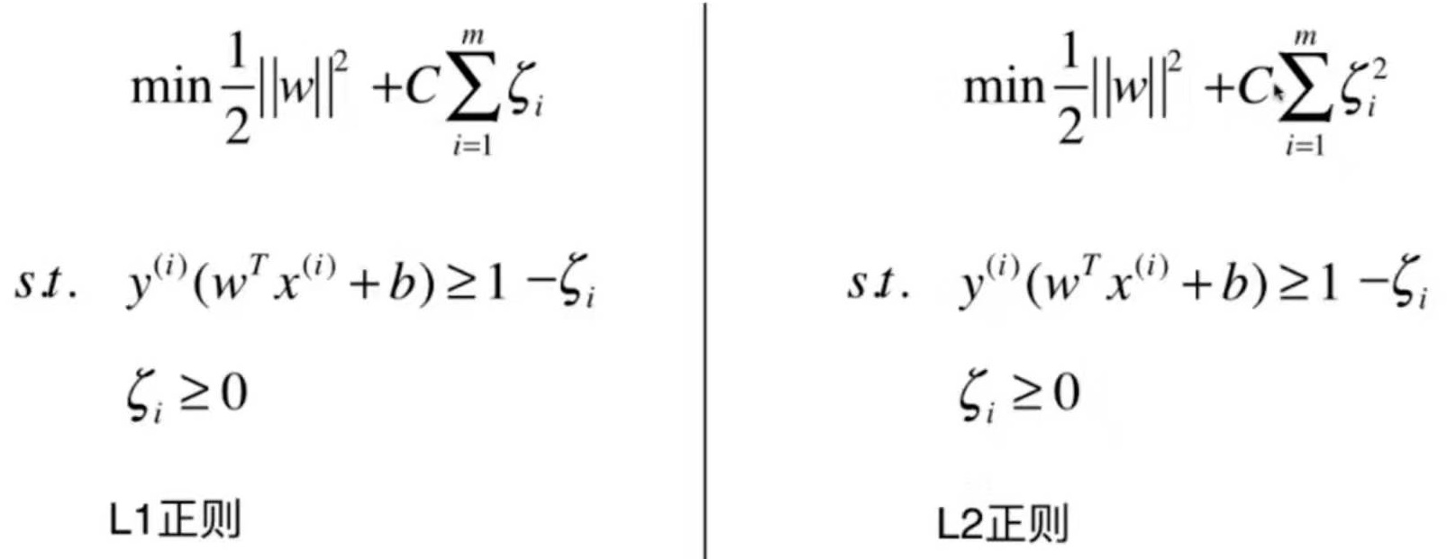
和KNN一样,使用SVM之前要做数据标准化处理,因为SVM算法涉及距离。
尺度不平衡的例子:

数据标准化之后:
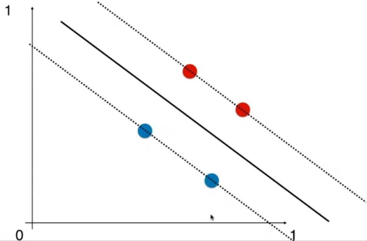
准备数据
import numpy as np
import matplotlib.pyplot as plt
from sklearn import datasets
iris = datasets.load_iris()
X = iris.data
y = iris.target
X = X[y<2,:2]
y = y[y<2]
plt.scatter(X[y==0,0],X[y==0,1], color='red')
plt.scatter(X[y==1,0],X[y==1,1], color='blue')
plt.show()
数据标准化
from sklearn.preprocessing import StandardScaler
standardScaler = StandardScaler()
standardScaler.fit(X)
X_standard = standardScaler.transform(X)
训练hard SVN模型
from sklearn.svm import LinearSVC
# Support Vector Classifier
svc = LinearSVC(C=1e9) # C 越大,越hard
svc.fit(X_standard, y)
分类效果
def plot_decision_boundary(model, axis):
x0, x1 = np.meshgrid(
np.linspace(axis[0], axis[1], int((axis[1]-axis[0])*100)).reshape(-1,1),
np.linspace(axis[2], axis[3], int((axis[3]-axis[2])*100)).reshape(-1,1)
)
X_new = np.c_[x0.ravel(), x1.ravel()]
y_predict = model.predict(X_new)
zz = y_predict.reshape(x0.shape)
from matplotlib.colors import ListedColormap
custom_cmap = ListedColormap(['#EF9A9A','#FFF59D','#90CAF9'])
plt.contourf(x0, x1, zz, cmap=custom_cmap)
plot_decision_boundary(svc, axis=[-3,3,-3,3])
plt.scatter(X_standard[y==0,0],X_standard[y==0,1], color='red')
plt.scatter(X_standard[y==1,0],X_standard[y==1,1], color='blue')
plt.show()
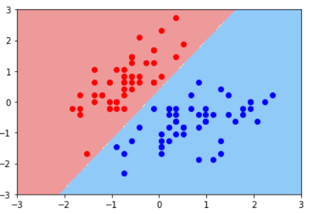
训练soft SVN 模型
svc2 = LinearSVC(C=0.01)
svc2.fit(X_standard, y)
plot_decision_boundary(svc2, axis=[-3,3,-3,3])
plt.scatter(X_standard[y==0,0],X_standard[y==0,1], color='red')
plt.scatter(X_standard[y==1,0],X_standard[y==1,1], color='blue')
plt.show()
 图中有一个点被错误地分类了,这是soft的效果
绘制margin
输入:svc.coef_
输出:array([[ 4.03240038, -2.50701084]])
样本中有两个特征,所以有2个系数,每个特征对应一个
输出是一个二维数组,因为sklearn提供的SVM算法可以处理多分类问题
输入:svc.intercept_
输出:array([0.92736326])
def plot_svc_decision_boundary(model, axis):
x0, x1 = np.meshgrid(
np.linspace(axis[0], axis[1], int((axis[1]-axis[0])*100)).reshape(-1,1),
np.linspace(axis[2], axis[3], int((axis[3]-axis[2])*100)).reshape(-1,1)
)
X_new = np.c_[x0.ravel(), x1.ravel()]
y_predict = model.predict(X_new)
zz = y_predict.reshape(x0.shape)
from matplotlib.colors import ListedColormap
custom_cmap = ListedColormap(['#EF9A9A','#FFF59D','#90CAF9'])
plt.contourf(x0, x1, zz, cmap=custom_cmap)
# 取出model的系数,只取第0个决策边界
w = model.coef_[0]
b = model.intercept_[0]
# 决策边界的直线方程:w0 * x0 + x1 * x1 + b = 0
# 决策边界的斜率和截距 => x1 = -w0/w1 * x0 - b/w1
plot_x = np.linspace(axis[0], axis[1], 200) # 绘制用的x
up_y = -w[0]/w[1] * plot_x - b/w[1] + 1/w[1] # w0 * x0 + x1 * x1 + b = 1
down_y = -w[0]/w[1] * plot_x - b/w[1] - 1/w[1] # w0 * x0 + x1 * x1 + b = -1
# 过滤,防止y超出图像边界
up_index = (up_y >= axis[2]) & (up_y <= axis[3])
down_index = (down_y >= axis[2]) & (down_y <= axis[3])
plt.plot(plot_x[up_index], up_y[up_index], color='black')
plt.plot(plot_x[down_index], down_y[down_index], color='black')
svc的margin
plot_svc_decision_boundary(svc, axis=[-3,3,-3,3])
plt.scatter(X_standard[y==0,0],X_standard[y==0,1], color='red')
plt.scatter(X_standard[y==1,0],X_standard[y==1,1], color='blue')
plt.show()
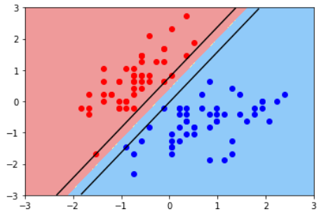
svc2的margin
plot_svc_decision_boundary(svc2, axis=[-3,3,-3,3])
plt.scatter(X_standard[y==0,0],X_standard[y==0,1], color='red')
plt.scatter(X_standard[y==1,0],X_standard[y==1,1], color='blue')
plt.show()
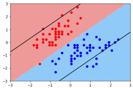
Note 1:sklarn提供的SVM算法支持多分类,默认使用ovr算法 Note 2:sklarn提供的SVM算法支持正则化,默认使用L2范式
import numpy as np
import matplotlib.pyplot as plt
from sklearn import datasets
X, y = datasets.make_moons()
# X.shape = (100, 2)
# y.shape = (100,)
plot_decision_boundary(poly_svc, axis=[-1.5,2.5,-1.0,1.5])
plt.scatter(X[y==0,0],X[y==0,1])
plt.scatter(X[y==1,0],X[y==1,1])
plt.show()

X, y = datasets.make_moons(noise=0.15, random_state=666) # 0.15可以理解为标准差
plt.scatter(X[y==0,0],X[y==0,1])
plt.scatter(X[y==1,0],X[y==1,1])
plt.show()

使用多项式特征的SVM
训练模型
from sklearn.preprocessing import PolynomialFeatures, StandardScaler
from sklearn.svm import LinearSVC
from sklearn.pipeline import Pipeline
def PolynomialSVC(degree, C=1.0):
return Pipeline([
('poly', PolynomialFeatures(degree=degree)),
('std_scaler', StandardScaler()),
('linearSVC', LinearSVC(C=C))
])
poly_svc = PolynomialSVC(degree=3)
poly_svc.fit(X, y)
绘制模型
def plot_decision_boundary(model, axis):
x0, x1 = np.meshgrid(
np.linspace(axis[0], axis[1], int((axis[1]-axis[0])*100)).reshape(-1,1),
np.linspace(axis[2], axis[3], int((axis[3]-axis[2])*100)).reshape(-1,1)
)
X_new = np.c_[x0.ravel(), x1.ravel()]
y_predict = model.predict(X_new)
zz = y_predict.reshape(x0.shape)
from matplotlib.colors import ListedColormap
custom_cmap = ListedColormap(['#EF9A9A','#FFF59D','#90CAF9'])
plt.contourf(x0, x1, zz, cmap=custom_cmap)
plot_decision_boundary(poly_svc, axis=[-1.5,2.5,-1.0,1.5])
plt.scatter(X[y==0,0],X[y==0,1])
plt.scatter(X[y==1,0],X[y==1,1])
plt.show()

使用多项式核函数的SVM
from sklearn.preprocessing import StandardScaler
from sklearn.svm import SVC
from sklearn.pipeline import Pipeline
def PolynomialKernelSVC(degree, C=1.0):
return Pipeline([
('std_scaler', StandardScaler()),
('kernelSVC', SVC(C=C, kernel='poly', degree=degree))
])
poly_kernel_svc = PolynomialKernelSVC(degree=3)
poly_kernel_svc.fit(X, y)
plot_decision_boundary(poly_kernel_svc, axis=[-1.5,2.5,-1.0,1.5])
plt.scatter(X[y==0,0],X[y==0,1])
plt.scatter(X[y==1,0],X[y==1,1])
plt.show()
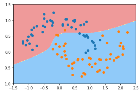

这是11-3中推导出来的公式。MVC本质上是这样的一个带条件的最优化问题。
在求解这个问题的过程要,要把公式变形:
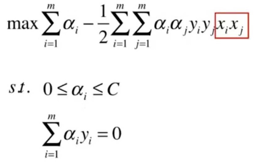
公式中红框标出来的部分,配合前面了两层累加符号,表示样本中任意两个x相乘。
所谓的给SVM增加多项式,就是:

把x做一些变形得到x',并且用x'代替公式中的x
核函数的思想是:有没有可能不显式地将x转换成x',而是直接使用一个函数得到

那么SVM的目标函数就可以写成:
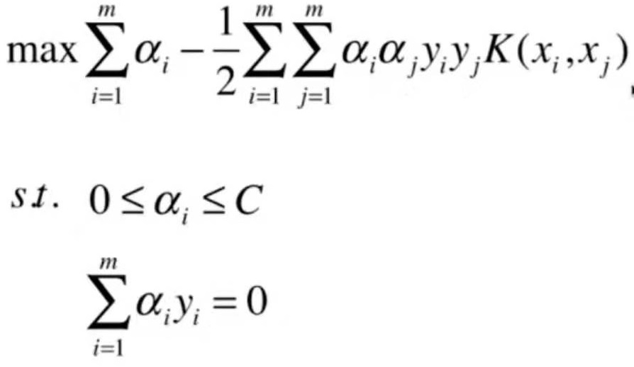
K函数 = Kernel function = Kernel trick
优点:1.节省了存储空间2.计算量变少
核函数本身不是SVM独有的技巧。只要算法转成了最优化问题,并且在求解最优化问题的过程中存在xi * xj或者类似这样的式子,都可以应该核函数技巧。
多项式核函数
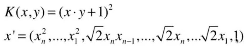
相当于给原来的x添加了二次项。
系数前面的常数项根号2不会影响模型的训练效果。
多项式的核函数:

下图是sklearn的SVM的文档,当核函数指定为poly时,degree相当于公式中的d,coef0相当于公式中的c
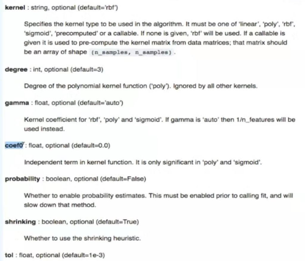
线性核函数:K(x, y) = x * y
K(x, y)表示x和y的点乘。高斯核函数的公式为:
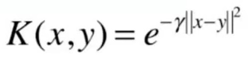
公式中的$$\gamma$$是高斯核函数中唯一的超参数。
高斯核函数 = RBF核 = Radial Basis Function Kernel = 镜像基函数
高斯核函数本质是将每个样本点映射到一个无穷维的特征空间
多项式特征为什么能处理线性不可分的问题?
依靠升维使得原本线性不可分的数据线性可分
例如有一组原本线性不可分的一维数据:

给数据增加一个内容为x^2的维度,数据就变成了这样:
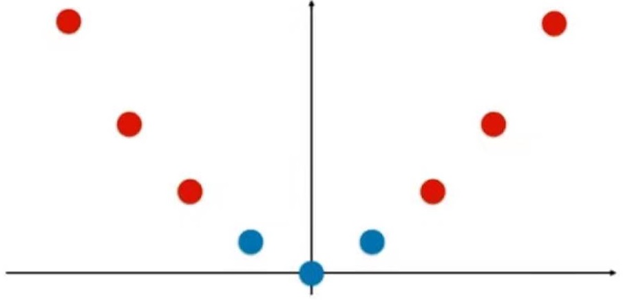 现在很容易找到一根直线把两类数据区分开:
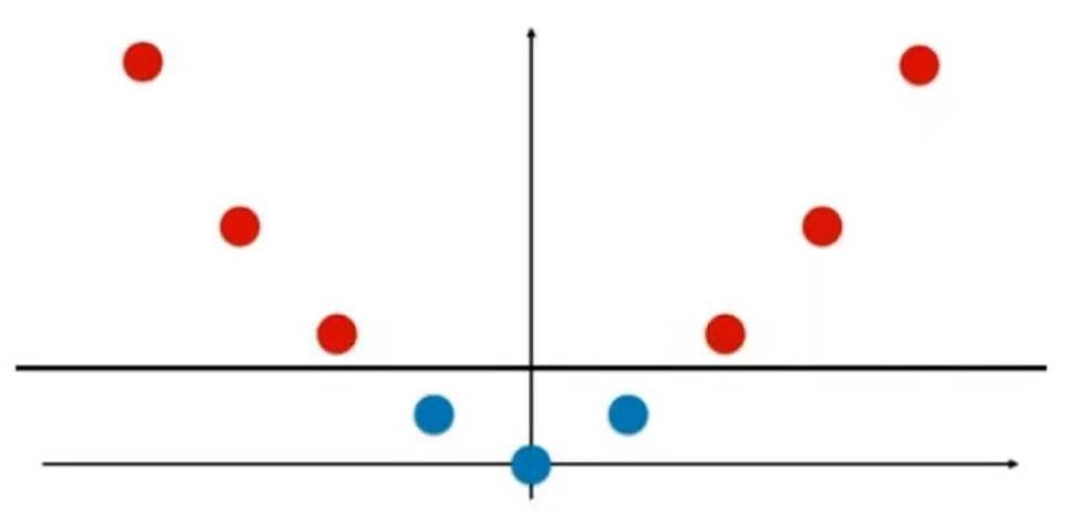
使用高斯核函数升维
再来看复用高斯核函数的例子。为了方便可视化,将原K做一些改变。
在原K中,是x相对y的映射,改成x相对两个固定的点的映射。
这两个固定的点就是图中的三角形位置。 l:landmark,地标
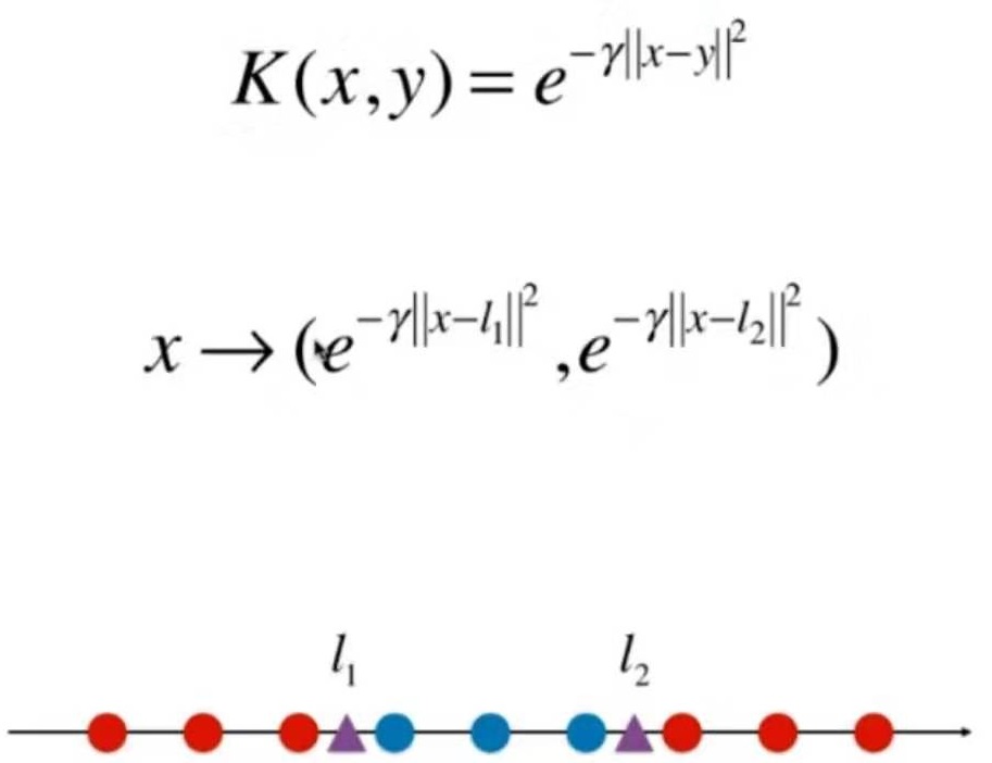
代码模拟高斯核函数的映射效果
import numpy as np
import matplotlib.pyplot as plt
x = np.arange(-4, 5, 1) # x = array([-4, -3, -2, -1, 0, 1, 2, 3, 4])
y = np.array((x>=-2) & (x<=2), dtype='int') # y = array([0, 0, 1, 1, 1, 1, 1, 0, 0])
plt.scatter(x[y==0], [0]*len(x[y==0]))
plt.scatter(x[y==1], [0]*len(x[y==1]))
plt.show()
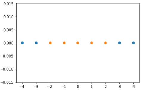
def gaussian(x, l):
gamma = 1.0
return np.exp(-gamma * (x-l)**2)
l1, l2 = -1, 1
X_new = np.empty((len(x),2))
for i, data in enumerate(x):
X_new[i, 0] = gaussian(data, l1)
X_new[i, 1] = gaussian(data, l2)
plt.scatter(X_new[y==0,0], X_new[y==0,1])
plt.scatter(X_new[y==1,0], X_new[y==1,1])
plt.show()
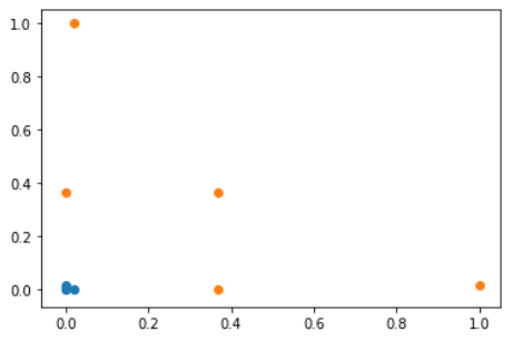
这样就得到了一个线性可分的结果:

解释
在这个例子中,使用图中的公式2来对x做映射,公式中的l1和l2是地标。
但实际的高斯公式是公式1,公式中的y是每一个数据点,也就是说,在高斯核函数中,每个样本都是一个地标landmark。它将m*n的数据映射成了m*m的数据。
使用高斯核函数训练样本,计算量非常大,训练时间也很长。
当m < n时,适用使用高斯核函数,例如自然语言处理。
gamma参数的意义
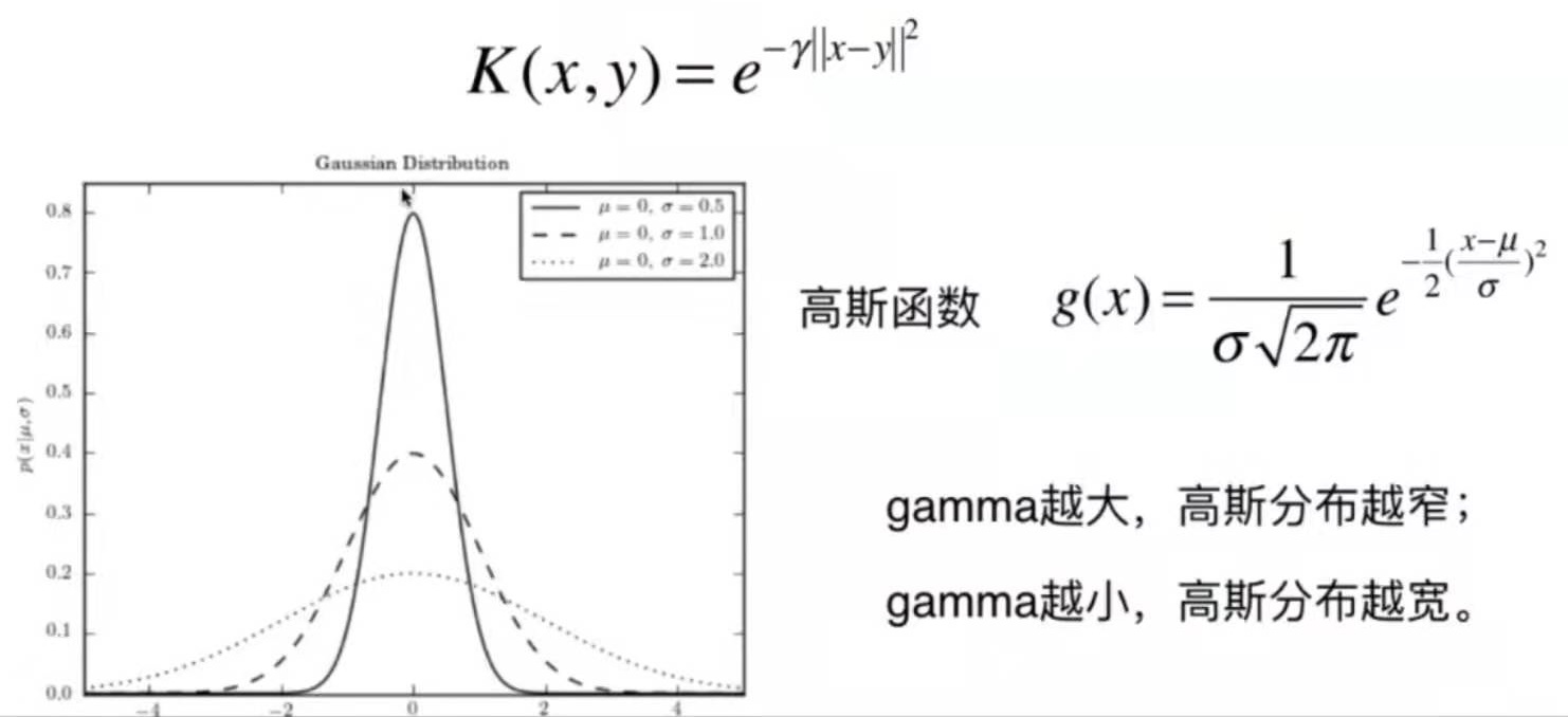
加载数据
import numpy as np
import matplotlib.pyplot as plt
from sklearn import datasets
X, y = datasets.make_moons()
X, y = datasets.make_moons(noise=0.15, random_state=666)
plt.scatter(X[y==0,0],X[y==0,1])
plt.scatter(X[y==1,0],X[y==1,1])
plt.show()
训练高斯核的SVM
from sklearn.preprocessing import StandardScaler
from sklearn.svm import SVC
from sklearn.pipeline import Pipeline
def RBFKernelSVC(gamma=1.0):
return Pipeline([
('std_scaler', StandardScaler()),
('rbfSVC', SVC(kernel='rbf', gamma= gamma))
])
svc = PolynomialKernelSVC()
svc.fit(X, y)
绘制决策边界
def plot_decision_boundary(model, axis):
x0, x1 = np.meshgrid(
np.linspace(axis[0], axis[1], int((axis[1]-axis[0])*100)).reshape(-1,1),
np.linspace(axis[2], axis[3], int((axis[3]-axis[2])*100)).reshape(-1,1)
)
X_new = np.c_[x0.ravel(), x1.ravel()]
y_predict = model.predict(X_new)
zz = y_predict.reshape(x0.shape)
from matplotlib.colors import ListedColormap
custom_cmap = ListedColormap(['#EF9A9A','#FFF59D','#90CAF9'])
plt.contourf(x0, x1, zz, cmap=custom_cmap)
plot_decision_boundary(svc, axis=[-1.5,2.5,-1.0,1.5])
plt.scatter(X[y==0,0],X[y==0,1])
plt.scatter(X[y==1,0],X[y==1,1])
plt.show()

gamma取不同值的效果对比
| 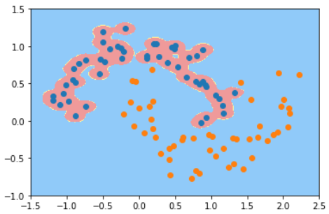 | 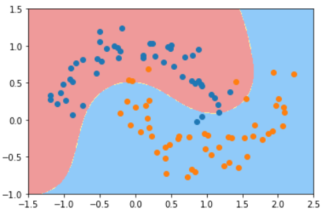 |  | 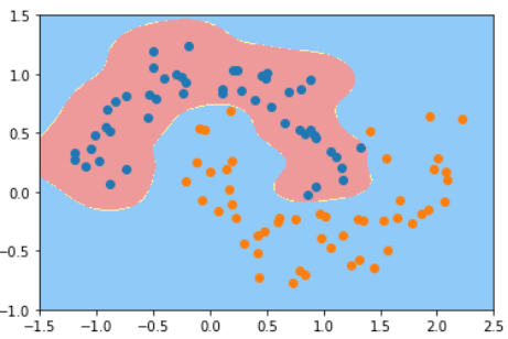 |
|---|---|---|---|---|
| gamma=1.0 | gamma=100 | gamma=0.5 | gamma=0.1 | gamma=10 |
可以把训练的效果看成是俯视这些样本点。某一类的每个样本点形成了一个以它为中心的正态分布。
gamma越大,这个分布的圈就越小。
回归问题是指找到一根直线/曲线最大程度的拟合样本点。
不同的回归算法对“拟合”有不同的理解。
例如线性回归算法定义“拟合”为:所有样本点到直线的MSE最小
而SVM将“拟合”定义为:尽可能多的点被包含在margin范围内,取margin中间的直线。(与解决分类问题相反的思路)
margin的距离为超参数
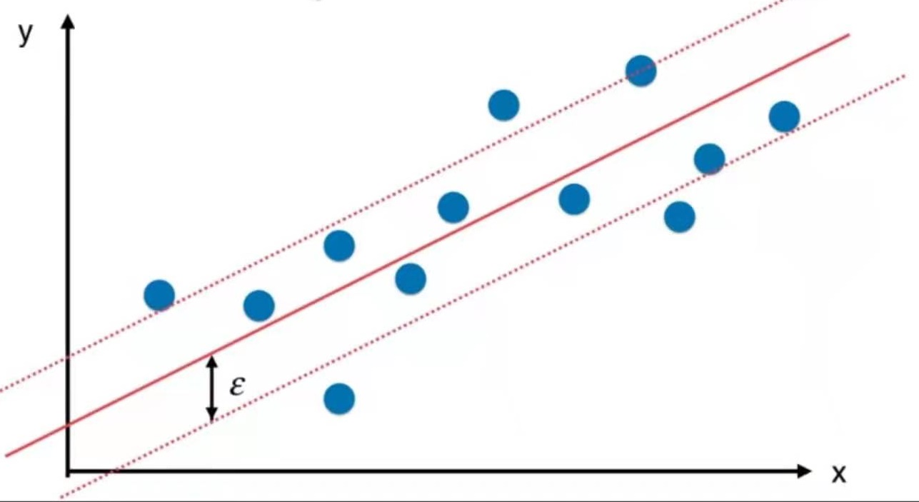
加载数据
import numpy as np
from sklearn import datasets
boston = datasets.load_boston()
x = boston.data
y = boston.target
from sklearn.model_selection import train_test_split
X_train, X_test, y_train, y_test = train_test_split(x, y, random_state=666)
训练模型
from sklearn.preprocessing import StandardScaler
from sklearn.svm import SVR
from sklearn.svm import LinearSVR
from sklearn.pipeline import Pipeline
# SVR = Support Vector Regression
# SVR和SVC的用法基本上一样
def StandardLinearSVR(epsilon=0.1):
return Pipeline([
('std_scaler', StandardScaler()),
('linearSVR', LinearSVR(epsilon=epsilon))
])
svr = StandardLinearSVR()
svr.fit(X_train, y_train)
svr.score(X_test, y_test)
输出结果:0.6358140020058993
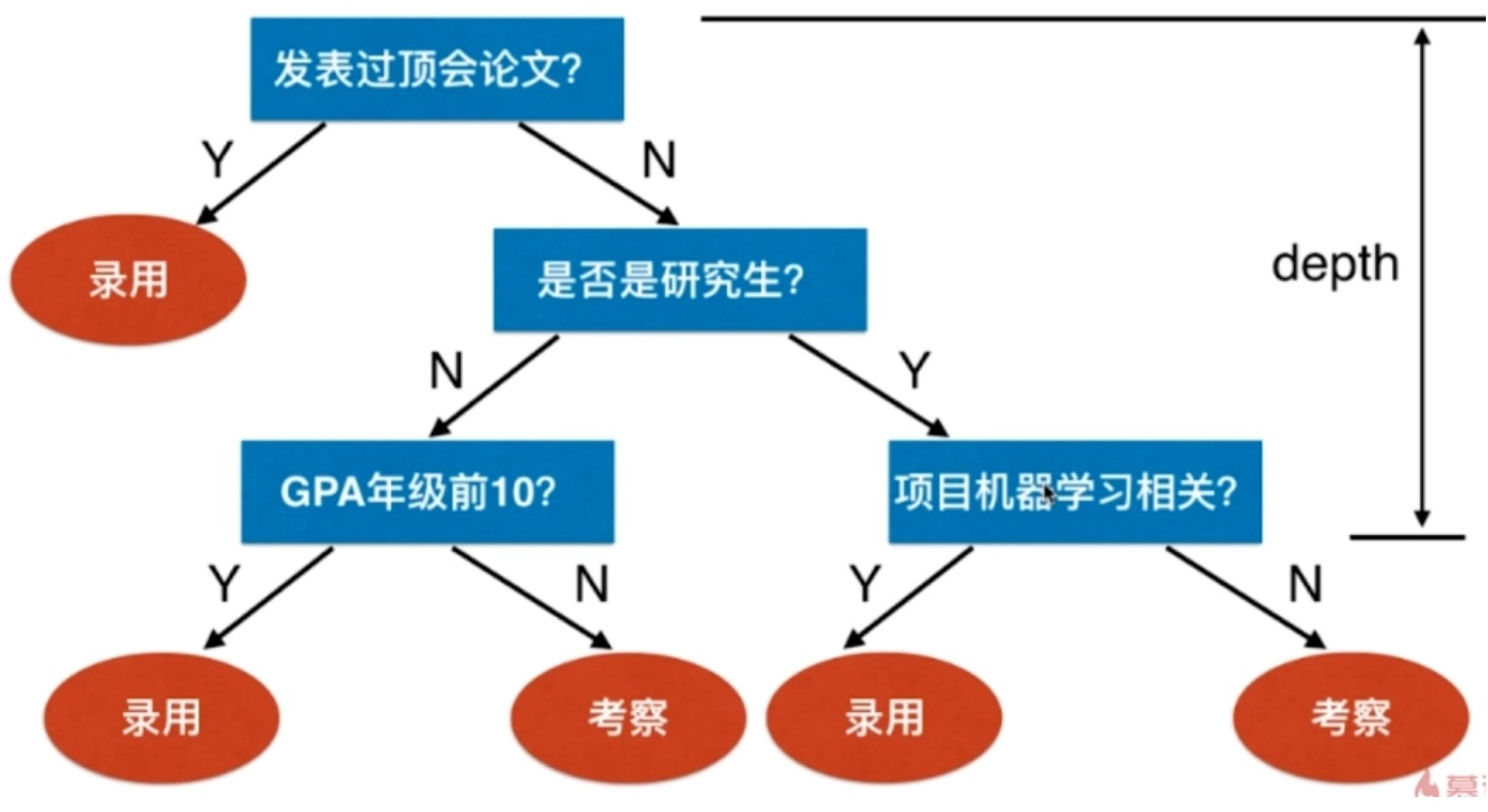 假设上图是某公司招聘算法工程师的过程。
图中的叶子节点代码决策,在寻找决策过程是形成了树是决策树。
这棵树的深度为3,因为最多经过3次判断就能做出决策。
使用sklearn中的决策树
import numpy as np
import matplotlib.pyplot as plt
from sklearn import datasets
iris = datasets.load_iris()
X = iris.data[:, 2:]
y = iris.target
plt.scatter(X[y==0,0],X[y==0,1])
plt.scatter(X[y==1,0],X[y==1,1])
plt.scatter(X[y==2,0],X[y==2,1])
plt.show()
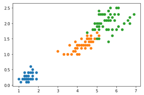
from sklearn.tree import DecisionTreeClassifier
dt_clf = DecisionTreeClassifier(max_depth=2, criterion='entropy') # entropy = 熵
dt_clf.fit(X, y)
plot_decision_boundary(dt_clf, axis=[0.5, 7.5, 0, 3])
plt.scatter(X[y==0,0],X[y==0,1])
plt.scatter(X[y==1,0],X[y==1,1])
plt.scatter(X[y==2,0],X[y==2,1])
plt.show()
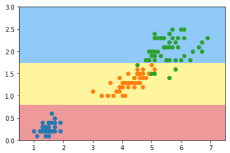
这个分类结果与视频中的分类结果不同
总结
决策树怎样做决策的
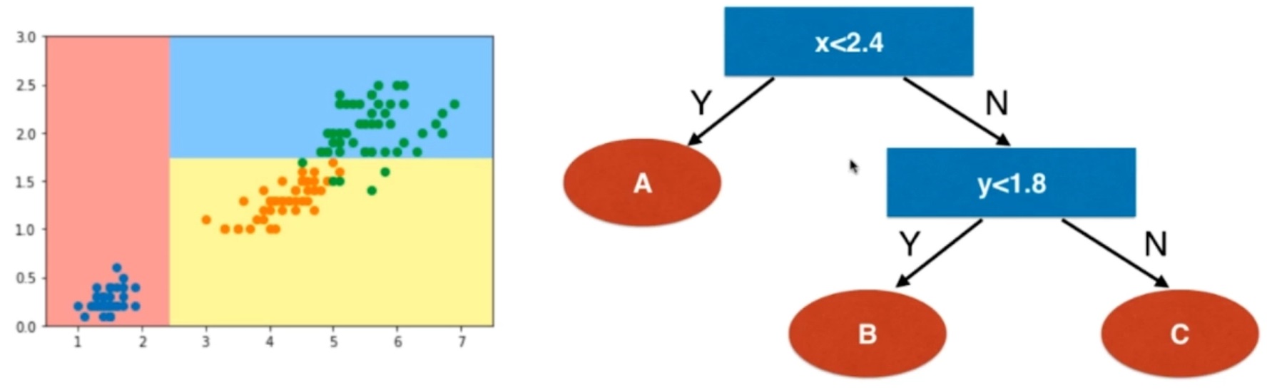 当属性是数值特征时,在每一个节点上,选择某一个维度上的数值,以它为域值将样本分成两类。
决策树的特点
- 是非参数学习算法
- 可以分类问题
- 天然可以解决多分类问题
- 也可以解决回归问题(用分类算法将样本归到某个叶子上,该叶子上所有样本的平均值即输出标记)
- 有非常好的可解释性
怎样创建决策树
- 每个结点在哪个维度做划分?
- 某个维度的哪个值上做划分?
假设上图是某公司招聘算法工程师的过程。
图中的叶子节点代码决策,在寻找决策过程是形成了树是决策树。
这棵树的深度为3,因为最多经过3次判断就能做出决策。
使用sklearn中的决策树
import numpy as np
import matplotlib.pyplot as plt
from sklearn import datasets
iris = datasets.load_iris()
X = iris.data[:, 2:]
y = iris.target
plt.scatter(X[y==0,0],X[y==0,1])
plt.scatter(X[y==1,0],X[y==1,1])
plt.scatter(X[y==2,0],X[y==2,1])
plt.show()
from sklearn.tree import DecisionTreeClassifier
dt_clf = DecisionTreeClassifier(max_depth=2, criterion='entropy') # entropy = 熵
dt_clf.fit(X, y)
plot_decision_boundary(dt_clf, axis=[0.5, 7.5, 0, 3])
plt.scatter(X[y==0,0],X[y==0,1])
plt.scatter(X[y==1,0],X[y==1,1])
plt.scatter(X[y==2,0],X[y==2,1])
plt.show()
这个分类结果与视频中的分类结果不同
总结
决策树怎样做决策的
当属性是数值特征时,在每一个节点上,选择某一个维度上的数值,以它为域值将样本分成两类。
决策树的特点
- 是非参数学习算法
- 可以分类问题
- 天然可以解决多分类问题
- 也可以解决回归问题(用分类算法将样本归到某个叶子上,该叶子上所有样本的平均值即输出标记)
- 有非常好的可解释性
怎样创建决策树
- 每个结点在哪个维度做划分?
- 某个维度的哪个值上做划分?
- 每个结点在哪个维度做划分?
- 某个维度的哪个值上做划分?
用信息熵解决以上问题
信息熵
信息熵表示一组变量的不确定度。
熵越大,不确定性越高。
熵越小,不确定性越低。
信息熵的计算公式:
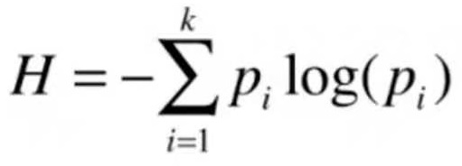
假设数据集中有三个类别,样本属于这三个类别的概率分别是{1/3, 1/3, 1/3},此时信息熵H为:
H = -1/3log(1/3) -1/3log(1/3) -1/3log(1/3) = 1.0986
如果三个类别的概率分别是{0.1、0.2、0.7},那么H=0.8018
如果三个类别的概率分别是{1, 0, 0},那么H=0
以二分类为例,画出信息熵的图像
数据只有两个类型,其中一类的概率为x,信息熵计算公式如下:
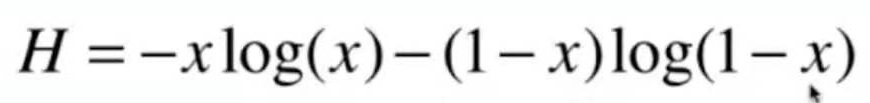
import numpy as np
import matplotlib.pyplot as plt
def entropy(p):
return -p * np.log(p) - (1-p) * np.log(1-p)
x = np.linspace(0.01, 0.99, 200)
plt.plot(x, entropy(x))
plt.show()

数据是任何一个类别的概率是一样大时,信息熵最大。
系统偏向于某一类,信息熵降低。
当数据100%确定是某一类时,信息熵为0
总结:
每一次划分时,让划分后的信息熵为所有划分结果的最低。
使用sklearn提供的接口
import numpy as np
import matplotlib.pyplot as plt
from sklearn import datasets
iris = datasets.load_iris()
X = iris.data[:, 2:]
y = iris.target
from sklearn.tree import DecisionTreeClassifier
dt_clf = DecisionTreeClassifier(max_depth=2, criterion='entropy')
dt_clf.fit(X, y)
def plot_decision_boundary(model, axis):
x0, x1 = np.meshgrid(
np.linspace(axis[0], axis[1], int((axis[1]-axis[0])*100)).reshape(-1,1),
np.linspace(axis[2], axis[3], int((axis[3]-axis[2])*100)).reshape(-1,1)
)
X_new = np.c_[x0.ravel(), x1.ravel()]
y_predict = model.predict(X_new)
zz = y_predict.reshape(x0.shape)
from matplotlib.colors import ListedColormap
custom_cmap = ListedColormap(['#EF9A9A','#FFF59D','#90CAF9'])
plt.contourf(x0, x1, zz, cmap=custom_cmap)
plot_decision_boundary(dt_clf, axis=[0.5, 7.5, 0, 3])
plt.scatter(X[y==0,0],X[y==0,1])
plt.scatter(X[y==1,0],X[y==1,1])
plt.scatter(X[y==2,0],X[y==2,1])
plt.show()

模拟使用信息熵进行划分
基于维度d上的值value对X和y进行划分
def split(X, y, d, value):
index_a = (X[:,d] <= value)
index_b = (X[:,d] > value)
return X[index_a], X[index_b], y[index_a], y[index_b]
计算划分后的每一组的熵
from collections import Counter
from math import log
def entropy(y):
counter = Counter(y) # counter是键值数据对,键是y的取值,值是y取这个键个数据
res = 0.0
for num in counter.values():
p = num / len(y)
res += -p * log(p)
return res
寻找熵最小的d和value
def try_split(X, y):
best_entropy = float('inf')
best_d, best_v = -1, -1
for d in range(X.shape[1]): # 穷搜每一个维度
sorted_index = np.argsort(X[:,d])
for i in range(1, len(X)): # 对每个样本遍历,可选的域值为两个点之间的值
if X[sorted_index[i-1], d] != X[sorted_index[i], d]:
v = (X[sorted_index[i-1], d] + X[sorted_index[i], d]) / 2
x_l, x_r, y_l, y_r = split(X, y, d, v)
e = entropy(y_l) + entropy(y_r)
if e < best_entropy:
best_entropy, best_d, best_v = e, d, v
return best_entropy, best_d, best_v
进行一次划分:
best_entropy, best_d, best_v = try_split(X, y)
print("best_entropy = ", best_entropy)
print("best_d = ", best_d)
print("best_v = ", best_v)
输出:
best_entropy = 0.6931471805599453
best_d = 0 # 代码横轴划分,表现是一根竖线
best_v = 2.45
与上面的图像结果不同,但与视频中的结果相同
存储划分结果:
X1_l, X1_r, y1_l, y1_r = split(X, y, best_d, best_v)
entropy(y1_l) = 0.0 # 左边只有一种数据,因此信息熵为0
entropy(y1_r) = 0.6931471805599453
左边已经不需要划分了,继续划分右边即可
best_entropy2, best_d2, best_v2 = try_split(X1_r, y1_r)
print("best_entropy = ", best_entropy2)
print("best_d = ", best_d2)
print("best_v = ", best_v2)
输出结果:
best_entropy = 0.4132278899361904
best_d = 1
best_v = 1.75
X2_l, X2_r, y2_l, y2_r = split(X1_r, y1_r, best_d2, best_v2)
entropy(y2_l) = 0.30849545083110386
entropy(y2_r) = 0.10473243910508653
两个结果都不为零,都可以继续划分
基尼系数的计算公式:
 其性质与信息熵相同。
基尼系数越大,不确定性越高。
基尼系数越小,不确定性越低。
以二分类为例,在二分类中,其中一类的概率为x,则G = -2x^2 + 2x
如果所有类别的概率相等时,基尼系数最大。类别确定时,基尼系数为0。
使用scikit learn中的基尼系数划分
import numpy as np
import matplotlib.pyplot as plt
from sklearn import datasets
iris = datasets.load_iris()
X = iris.data[:, 2:]
y = iris.target
from sklearn.tree import DecisionTreeClassifier
dt_clf = DecisionTreeClassifier(max_depth=2, criterion='gini')
dt_clf.fit(X, y)
def plot_decision_boundary(model, axis):
x0, x1 = np.meshgrid(
np.linspace(axis[0], axis[1], int((axis[1]-axis[0])*100)).reshape(-1,1),
np.linspace(axis[2], axis[3], int((axis[3]-axis[2])*100)).reshape(-1,1)
)
X_new = np.c_[x0.ravel(), x1.ravel()]
y_predict = model.predict(X_new)
zz = y_predict.reshape(x0.shape)
from matplotlib.colors import ListedColormap
custom_cmap = ListedColormap(['#EF9A9A','#FFF59D','#90CAF9'])
plt.contourf(x0, x1, zz, cmap=custom_cmap)
plot_decision_boundary(dt_clf, axis=[0.5, 7.5, 0, 3])
plt.scatter(X[y==0,0],X[y==0,1])
plt.scatter(X[y==1,0],X[y==1,1])
plt.scatter(X[y==2,0],X[y==2,1])
plt.show()
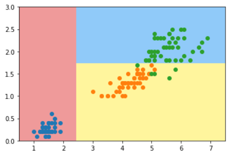
模拟使用基尼系数进行划分
代码和14-3基本上一样
from collections import Counter
from math import log
def split(X, y, d, value):
index_a = (X[:,d] <= value)
index_b = (X[:,d] > value)
return X[index_a], X[index_b], y[index_a], y[index_b]
def gini(y):
counter = Counter(y)
res = 1.0
for num in counter.values():
p = num / len(y)
res -= p ** 2
return res
def try_split(X, y):
best_gini = float('inf')
best_d, best_v = -1, -1
for d in range(X.shape[1]):
sorted_index = np.argsort(X[:,d])
for i in range(1, len(X)):
if X[sorted_index[i-1], d] != X[sorted_index[i], d]:
v = (X[sorted_index[i-1], d] + X[sorted_index[i], d]) / 2
x_l, x_r, y_l, y_r = split(X, y, d, v)
e = gini(y_l) + gini(y_r)
if e < best_gini:
best_gini, best_d, best_v = e, d, v
return best_gini, best_d, best_v
进行一次划分:
best_g, best_d, best_v = try_split(X, y)
print("best_g = ", best_g)
print("best_d = ", best_d)
print("best_v = ", best_v)
输出:
best_g = 0.5
best_d = 0 # 代码横轴划分,表现是一根竖线
best_v = 2.45
存储划分结果:
X1_l, X1_r, y1_l, y1_r = split(X, y, best_d, best_v)
gini(y1_l) = 0.0 # 左边只有一种数据,因此信息熵为0
gini(y1_r) = 0.5
左边已经不需要划分了,继续划分右边即可
best_g2, best_d2, best_v2 = try_split(X1_r, y1_r)
print("best_g = ", best_g2)
print("best_d = ", best_d2)
print("best_v = ", best_v2)
输出结果:
best_g = 0.2105714900645938
best_d = 1
best_v = 1.75
X2_l, X2_r, y2_l, y2_r = split(X1_r, y1_r, best_d2, best_v2)
gini(y2_l) = 0.1680384087791495
gini(y2_r) = 0.04253308128544431
信息熵 VS 基尼系数
信息熵计算比基尼系数稍慢。
scikit-learn中默认使用基尼系数。
大多数时候二者没有特别的效果优劣。
决策树又叫CART
CART = Classification And Regression Tree
根据某一个维度v和某一个域值d进行二分,这样得到的树就叫CART
scikit-learn创建决策树的方法就叫CART。
还有其它创建决策树的方法,例如ID3、C4.5、C5.0
创建好决策树好,预测一个样本的时间复杂度为O(log(m))
训练模型的时间复杂度为:O(nmlog(m))
是非参数学习算法,非常容易产生过拟合。
实际使用决策树时都要进行剪枝,1.降低复杂度2.解决过拟合
决策树使用不同的超参数的结果对比
生成数据
import numpy as np
import matplotlib.pyplot as plt
from sklearn import datasets
X, y = datasets.make_moons(noise=0.25, random_state=666)
plt.scatter(X[y==0,0],X[y==0,1])
plt.scatter(X[y==1,0],X[y==1,1])
plt.show()
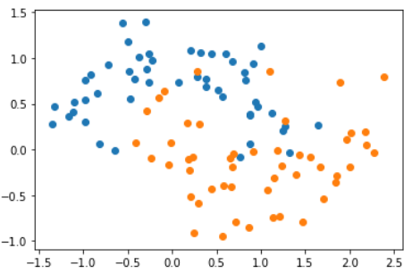
使用默认参数训练
from sklearn.tree import DecisionTreeClassifier
# 默认情况下使用gini系数,且一直向下划分到所有gini系数都是0为止
dt_clf = DecisionTreeClassifier()
dt_clf.fit(X, y)
def plot_decision_boundary(model, axis):
x0, x1 = np.meshgrid(
np.linspace(axis[0], axis[1], int((axis[1]-axis[0])*100)).reshape(-1,1),
np.linspace(axis[2], axis[3], int((axis[3]-axis[2])*100)).reshape(-1,1)
)
X_new = np.c_[x0.ravel(), x1.ravel()]
y_predict = model.predict(X_new)
zz = y_predict.reshape(x0.shape)
from matplotlib.colors import ListedColormap
custom_cmap = ListedColormap(['#EF9A9A','#FFF59D','#90CAF9'])
plt.contourf(x0, x1, zz, cmap=custom_cmap)
plot_decision_boundary(dt_clf, axis=[-1.5, 2.5, -1.0, 1.5])
plt.scatter(X[y==0,0],X[y==0,1])
plt.scatter(X[y==1,0],X[y==1,1])
plt.scatter(X[y==2,0],X[y==2,1])
plt.show()
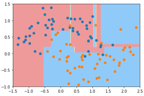 典型的过拟合
使用不同的超参数的结果对比
| default | max_depth=2 | min_samples_split=10 | min_samples_leaf=6 | max_leaf_nodes=4 |
|---|---|---|---|---|
| 一直向下划分到所有gini系数都是0为止 | 最大深度 | 对于一个节点至少有多个样本才继续划分 | 叶子节点至少有几个样本 | 最多有多少个叶子 |
| 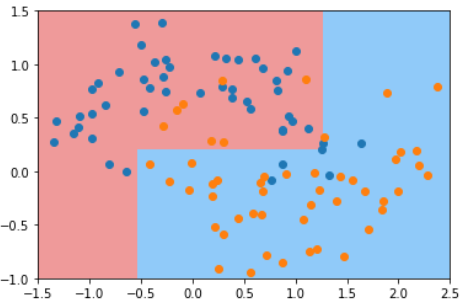 | 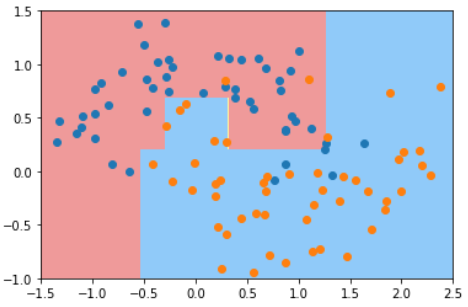 | 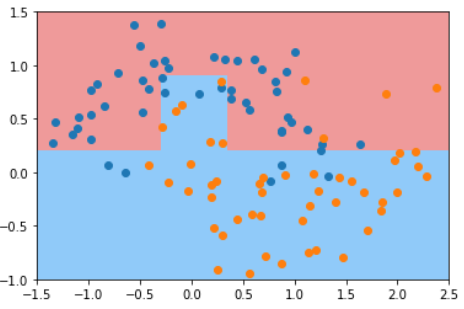 |  |
使用这些参数时:
- 避免欠拟合
- 使用风格搜索来组合这些参数
回归问题是指找到一根直线/曲线最大程度的拟合样本点。
不同的回归算法对“拟合”有不同的理解。
例如线性回归算法定义“拟合”为:所有样本点到直线的MSE最小
而SVM将“拟合”定义为:尽可能多的点被包含在margin范围内,取margin中间的直线。(与解决分类问题相反的思路)
margin的距离为超参数
代码实现
import numpy as np
from sklearn import datasets
boston = datasets.load_boston()
x = boston.data
y = boston.target
from sklearn.model_selection import train_test_split
X_train, X_test, y_train, y_test = train_test_split(x, y, random_state=666)
from sklearn.tree import DecisionTreeRegressor
dt_reg = DecisionTreeRegressor()
dt_reg.fit(X_train, y_train)
dt_reg.score(X_test, y_test) # 0.6872676909790005
dt_reg.score(X_train, y_train) # 1.0
训练数据集上预测的准确率是100%,而在测试数据集上效果不好。 决策树非常容易产生过拟合现象,要消除过拟合就要使用12-5中介绍的参数。
- 决策树的边界都是与某个轴平行的。
场景1:
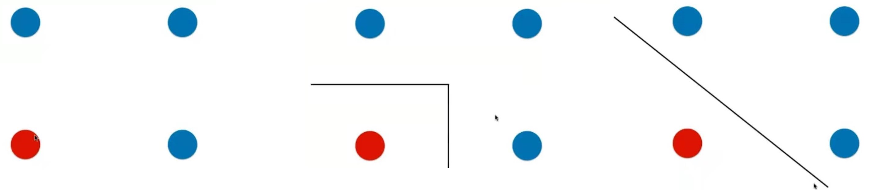
对于图中这样的数据点,决策树给出的决策边界可能是中间这样的,而右边这样的决策边界可能是更好的 场景2:
对于这些情况可以很好的划分,但如果对数据稍微做一些旋转,划分结果就不一样了,

- 高度依赖于参数,对样本敏感
- 在之前的训练中得到这样的决策边界
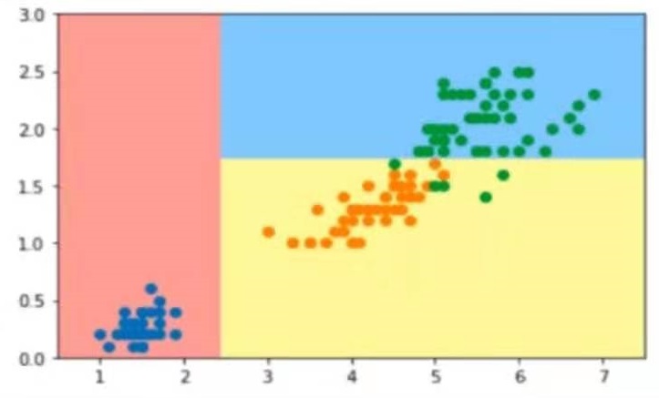 但如果去掉其中一个点,可能就会得到这样的的决策边界

决策树本身并不能很好的分类,但它是决策森林的基础。使用决策森林能得到很好的结果。
多种机器学习算法都能做同样的事情。让不同的算法针对同一个数据都跑一遍,最终使用投票的方法,少数服从多数,用多数投票的结果作为最终的结果。
import numpy as np
import matplotlib.pyplot as plt
from sklearn import datasets
X, y = datasets.make_moons(noise=0.25, random_state=666)
from sklearn.model_selection import train_test_split
X_train, X_test, y_train, y_test = train_test_split(X, y, random_state=42)
plt.scatter(X[y==0,0],X[y==0,1])
plt.scatter(X[y==1,0],X[y==1,1])
plt.show()

自己实现集成学习
逻辑回归
from sklearn.linear_model import LogisticRegression
log_clf = LogisticRegression()
log_clf.fit(X_train, y_train)
log_clf.score(X_test, y_test)
输出:0.864
SVM
from sklearn.svm import SVC
svm_clf = SVC()
svm_clf.fit(X_train, y_train)
svm_clf.score(X_test, y_test)
输出:0.888
决策树
from sklearn.tree import DecisionTreeClassifier
dt_clf = DecisionTreeClassifier()
dt_clf.fit(X_train, y_train)
dt_clf.score(X_test, y_test)
输出:0.84
集成学习
y_predict1 = log_clf.predict(X_test)
y_predict2 = svm_clf.predict(X_test)
y_predict3 = dt_clf.predict(X_test)
y_predict = np.array((y_predict1+y_predict2+y_predict3) >= 2, dtype='int')
from sklearn.metrics import accuracy_score
accuracy_score(y_test, y_predict)
输出:0.896
使用集成学习方法提高了准确率
使用Voting Classifier
from sklearn.ensemble import VotingClassifier
voting_clf = VotingClassifier(estimators=[
('log_clf', LogisticRegression()),
('svm_clf', SVC()),
('dt_clf', DecisionTreeClassifier())
], voting='hard')
voting_clf.fit(X_train, y_train)
voting_clf.score(X_test, y_test)
输出:0.896
多种机器学习算法都能做同样的事情。让不同的算法针对同一个数据都跑一遍,最终使用投票的方法,少数服从多数,用多数投票的结果作为最终的结果。
import numpy as np
import matplotlib.pyplot as plt
from sklearn import datasets
X, y = datasets.make_moons(noise=0.25, random_state=666)
from sklearn.model_selection import train_test_split
X_train, X_test, y_train, y_test = train_test_split(X, y, random_state=42)
plt.scatter(X[y==0,0],X[y==0,1])
plt.scatter(X[y==1,0],X[y==1,1])
plt.show()
自己实现集成学习
逻辑回归
from sklearn.linear_model import LogisticRegression
log_clf = LogisticRegression()
log_clf.fit(X_train, y_train)
log_clf.score(X_test, y_test)
输出:0.864
SVM
from sklearn.svm import SVC
svm_clf = SVC()
svm_clf.fit(X_train, y_train)
svm_clf.score(X_test, y_test)
输出:0.888
决策树
from sklearn.tree import DecisionTreeClassifier
dt_clf = DecisionTreeClassifier()
dt_clf.fit(X_train, y_train)
dt_clf.score(X_test, y_test)
输出:0.84
集成学习
y_predict1 = log_clf.predict(X_test)
y_predict2 = svm_clf.predict(X_test)
y_predict3 = dt_clf.predict(X_test)
y_predict = np.array((y_predict1+y_predict2+y_predict3) >= 2, dtype='int')
from sklearn.metrics import accuracy_score
accuracy_score(y_test, y_predict)
输出:0.896
使用集成学习方法提高了准确率
使用Voting Classifier
from sklearn.ensemble import VotingClassifier
voting_clf = VotingClassifier(estimators=[
('log_clf', LogisticRegression()),
('svm_clf', SVC()),
('dt_clf', DecisionTreeClassifier())
], voting='hard')
voting_clf.fit(X_train, y_train)
voting_clf.score(X_test, y_test)
输出:0.896
更合理的投票,应该有权值。
假如一个二分类问题,5个模型分别对一个样本进行分类。以下是每个模型认为每种分类的概率:
模型1:A-99%,B-1%
模型2:A-49%,B-51%
模型3:A-40%,B-60%
模型4:A-90%,B-10%
模型5:A-30%,B-70%
按照hard voting,投票结果为B
但考虑上每种类的概率,投票结果为A
把每个分类的概率当作权值,就是soft voting
soft voting要求集合中的每一个模型都能估计概率
即有predict_proba这个函数
逻辑回归,KNN,决策树(叶子结点的每个类的比例),都能估计概率。
SVM本身没有考虑概率,因为它是计算margin。但SVM可以有一种方法来计算概率。
自己实现集成学习
使用13-1的数据:
Hard Voting Classifier
from sklearn.ensemble import VotingClassifier
from sklearn.ensemble import VotingClassifier
from sklearn.linear_model import LogisticRegression
from sklearn.svm import SVC
from sklearn.tree import DecisionTreeClassifier
voting_clf = VotingClassifier(estimators=[
('log_clf', LogisticRegression()),
('svm_clf', SVC()),
('dt_clf', DecisionTreeClassifier(random_state=666))
], voting='hard')
voting_clf.fit(X_train, y_train)
voting_clf.score(X_test, y_test)
输出:0.896
Soft Voting Classifier
from sklearn.ensemble import VotingClassifier
from sklearn.linear_model import LogisticRegression
from sklearn.svm import SVC
from sklearn.tree import DecisionTreeClassifier
voting_clf2 = VotingClassifier(estimators=[
('log_clf', LogisticRegression()),
('svm_clf', SVC(probability=True)),
('dt_clf', DecisionTreeClassifier(random_state=42))
], voting='soft')
voting_clf2.fit(X_train, y_train)
voting_clf2.score(X_test, y_test)
输出:0.92
虽然有很多机器学习的算法,但从投票的角度看,仍然不够多
创建更多的子模型,集成更多子模型的意见
子模型之间不能一致,子模型之间要有差异性
如果创建差异性?
解决方法:
每个子模型只看样本数据的一部分。
每个子模型不太需要太高的准确率。只要子模型足够多,准确率就会提高。
例如500个子模型,每个子模型的准确率是60%,最终准确率能达到99.9%
取样方法:
- 放回取样 bagging(bootstrap)
- 不放回取样 pasting
bagging更常用,优点:
- 没有那么依赖随机
- 数据量要求没那么高
使用13-1中的数据
from sklearn.tree import DecisionTreeClassifier
from sklearn.ensemble import BaggingClassifier
bagging_clf = BaggingClassifier(DecisionTreeClassifier(),n_estimators=500, max_samples=100, bootstrap=True)
# 决策树这种非参数的算法更容易产生差异较大的子模型
# 所有集成学习如果要集成成百上千个子模型,通常首先决策树
# n_estimators:子模型数
# max_samples:每个子模型看的样本树
# bootstrap:放回取样
bagging_clf.fit(X_train, y_train)
bagging_clf.score(X_test, y_test)
输出:0.912
bagging_clf2 = BaggingClassifier(DecisionTreeClassifier(),n_estimators=1000, max_samples=100, bootstrap=True)
bagging_clf2.fit(X_train, y_train)
bagging_clf2.score(X_test, y_test)
输出:0.92
OOB:out of bag
放回取样导致一部分样本很有可能没有取到。
平均大约有37%的样本没有取到。
不使用train_test_split,而是使用这部分没有取到的样本做测试/验证。
使用13-1中的数据,但不做train_test_split
from sklearn.tree import DecisionTreeClassifier
from sklearn.ensemble import BaggingClassifier
bagging_clf = BaggingClassifier(DecisionTreeClassifier(),n_estimators=500, max_samples=100, bootstrap=True, oob_score=True)
bagging_clf.fit(X, y)
bagging_clf.oob_score_
输出:0.918
bagging的思路极易并行化处理,n_jobs
针对特征进行随机采样: Random Subspaces
当样本的特征非常多的时使用这种方法,比如图像样本
既针对样本,又针对特征进行随机采样:Random Patches
Random Subspaces
random_subspaces_clf = BaggingClassifier(DecisionTreeClassifier(),n_estimators=500, max_samples=500, bootstrap=True, oob_score=True, n_jobs=-1, max_features=1, bootstrap_features=True)
random_subspaces_clf.fit(X, y)
random_subspaces_clf.oob_score_
输出:0.838
Random Patches
random_subspaces_clf = BaggingClassifier(DecisionTreeClassifier(),n_estimators=500, max_samples=100, bootstrap=True, oob_score=True, n_jobs=-1, max_features=1, bootstrap_features=True)
random_subspaces_clf.fit(X, y)
random_subspaces_clf.oob_score_
输出:0.874
Bagging
Base Estimator: Decision Tree
只要是以决策树为基础的集成学习算法都叫随机森林。
scikit-learn提供了随机森林算法,并为算法提供了更多的随机性。
sickit-learn中,决策树在节点上划分,在随机的特征子集上寻找最优划分的特征。
随机森林
使用13-1中的数据,但random_state=666
import numpy as np
import matplotlib.pyplot as plt
from sklearn import datasets
X, y = datasets.make_moons(n_samples=500, noise=0.3, random_state=666)
plt.scatter(X[y==0,0],X[y==0,1])
plt.scatter(X[y==1,0],X[y==1,1])
plt.show()

from sklearn.ensemble import RandomForestClassifier
rf_clf = RandomForestClassifier(n_estimators=500, random_state=666, oob_score=True)
rf_clf.fit(X, y)
rf_clf.oob_score_
输出:0.892
from sklearn.ensemble import RandomForestClassifier
rf_clf2 = RandomForestClassifier(n_estimators=500, max_leaf_nodes=16, random_state=666, oob_score=True)
rf_clf2.fit(X, y)
rf_clf2.oob_score_
输出:0.906
使用extra-tree
extra-tree = extreme random trees,极其随机的的随机树。
极其随机表现在:决策树在节点上划分,使用随机的特征的随机的阈值。
提供额外的随机性,抑制过拟合,但增大了bias
相对于随机森林,速度更快
from sklearn.ensemble import ExtraTreesClassifier
et_clf = ExtraTreesClassifier(n_estimators=500, bootstrap=True, oob_score=True, random_state=666)
et_clf.fit(X, y)
et_clf.oob_score_
输出:0.892
集成学习解决回归问题
from sklearn.ensemble import BaggingRegressor
from sklearn.ensemble import RandomForestRegressor
from sklearn.ensemble import ExtraTreesRegressor
一类集成学习的思路:独立地集成多个模型,让各种子模型在视角上有差异化,并最终综合这些子模型的结果,获得学习的最终结果。
另一类集成学习的思路叫做boosting。boosting即增强的意思。
boosting也要集成多个模型,但每个模型都在尝试增强(boosting)整体的效果。子模型之间不是独立的关系。
Ada Boosting
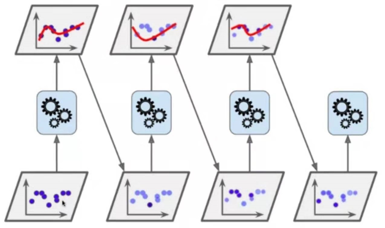
原始数据集1 --某个算法1--> 某个模型1
模型1没有很好学习的点的权值增大,很好学习到的点的权值减小,得到数据集2 --某个算法2 --> 某个模型2
。。。
每一个子模型都在推动上一个子模型犯的错误
用这些子模型投票得到最终结果
使用13-5中的数据
因为boosting算法没有oob_score,所以使用train_test_split测试算法
from sklearn.ensemble import AdaBoostClassifier
from sklearn.tree import DecisionTreeClassifier
# 使用决策树作为基础模型,决策树的参数在这里都能用
ada_clf = AdaBoostClassifier(DecisionTreeClassifier(max_depth=2), n_estimators=500)
ada_clf.fit(X_train, y_train)
ada_clf.score(X_test, y_test)
输出:0.864
Gradient Boosting
训练一个模型m1,产生错误e1
针对e1训练第二个模型m2,产生错误e2
针对e2训练第三个模型m3,产生错误e3
。。。
最终预测结果是m1+m2+m3+...
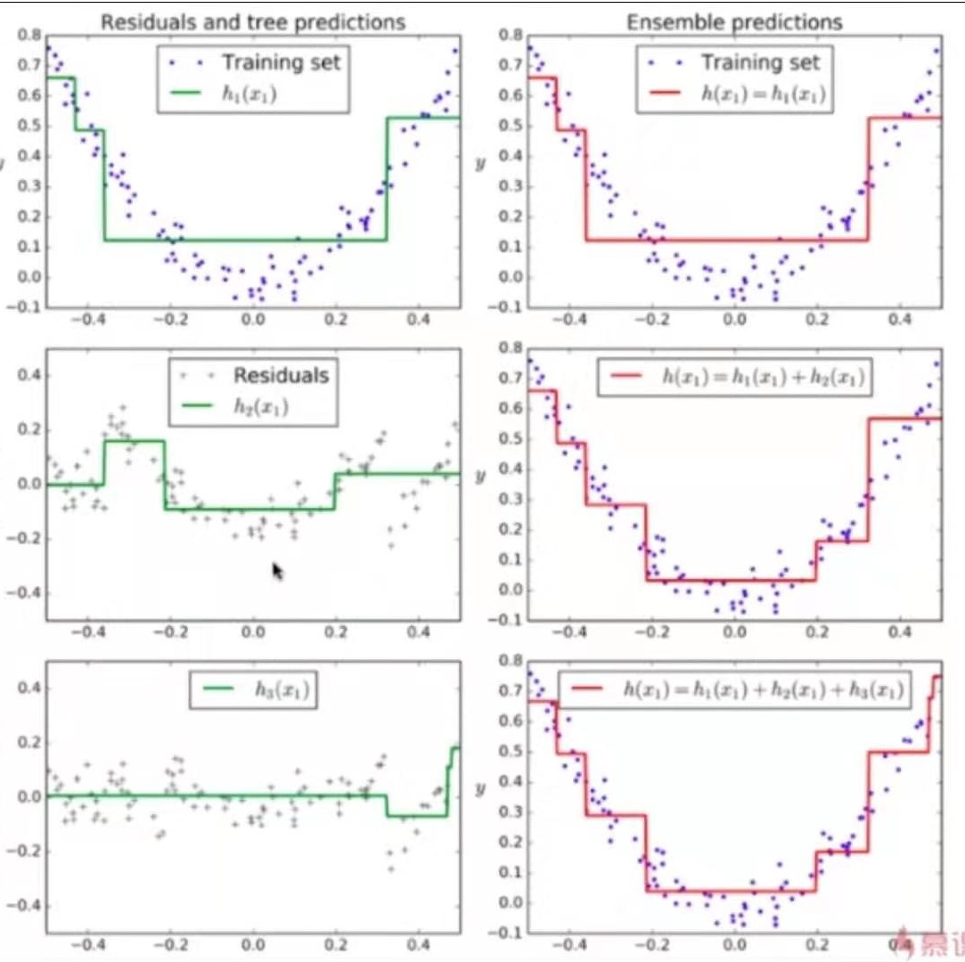
from sklearn.ensemble import GradientBoostingClassifier
# 指定以决策树为基础,不能选择
gd_clf = GradientBoostingClassifier(max_depth=2, n_estimators=500)
gd_clf.fit(X_train, y_train)
gd_clf.score(X_test, y_test)
输出:0.904
boosting解决回归问题
from sklearn.ensemble import AdaBoostRegressor
from sklearn.ensemble import GradientBoostingRegressor

stackgin的思路:假设使用三个算法分别得到机器学习的结果,但是不像前面那么直接将三个结果综合,而是用这三个算法作为输出,训练一个新的模型,使用这个模型的输出作为最终的输出。
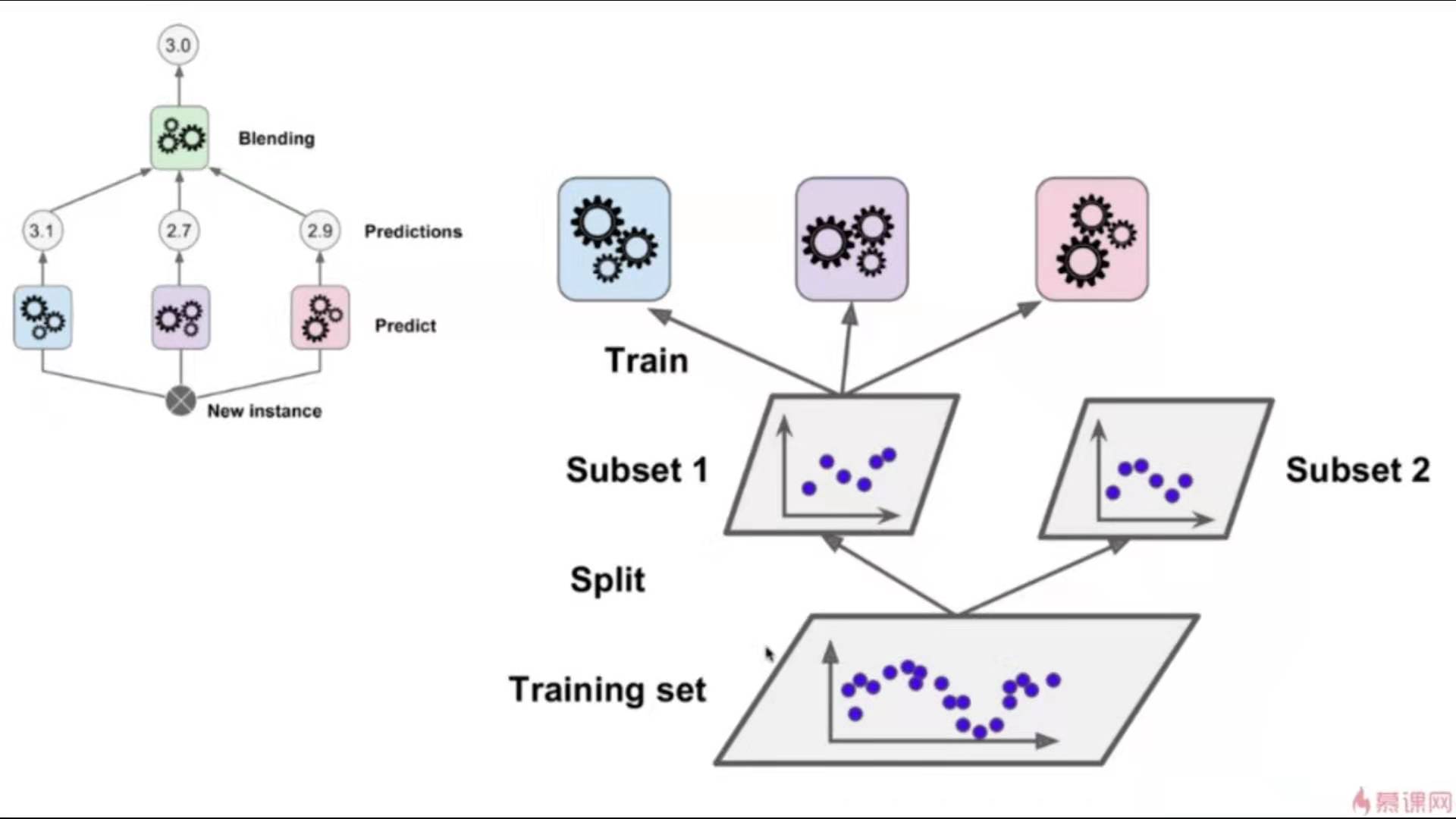
训练方法:将数据集分成2分,一份用于训练第一层的3个模型,第二份用于训练第二层的模型。最终得到整体模型。
这个模型还可以更复杂,比如:
 要训练这个模型需要把数据分成3份,每一份用于训练一层模型。
这样的模型非常容易过拟合。
这样的模型有点类似于神经网络。这是深度学习的范畴。
scikit-learn没有提供stacking模型的接口。