常规的梯度下降法，又叫批量梯度下降法，Batch Gradient Descent

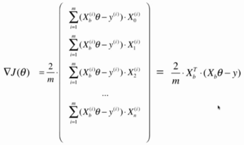
问题：当样本数m很大时会非常耗时

解决方法：每次只对其中一个样本做计算

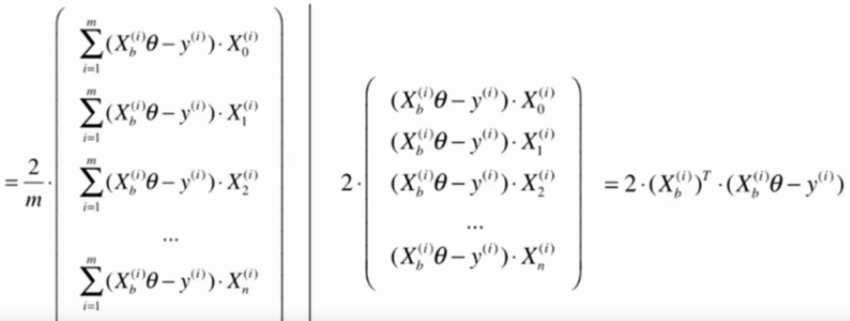
把去掉m后计算的公式作为搜索的方向。
由于不能保证这种方法计算得到的方向一定是损失最小的方向，甚至不能保证一定是损失函数减小的方向。也不能找到最小值的位置。
但仍然能到函数的最小值附近。
如果m非常大，可以用一定的精度来换时间。

在随机梯度下降法过程中，学习率很重要。
如果学习率取固定值，很有可以到了最小值附近后又跳出去了。
学习率应逐渐递减。（模拟退火的思想）

通常a取5，b取50

测试数据

import numpy as np
import matplotlib.pyplot as plt

m = 100000

x = np.random.normal(size=m)
X = x.reshape(-1, 1)
y = 4. * x + 3. + np.random.normal(0, 3, size=m)

批量梯度下降法

算法

def J(theta, X_b, y):
    try:
        return np.sum((y - X_b.dot(theta))**2) / len(X_b)
    except:
        return float('inf')

def dJ(theta, X_b, y):
    return X_b.T.dot(X_b.dot(theta)-y) * 2. / len(X_b)

def gradient_descent(X_b, y, initial_theta, eta, n_iters = 1e4, epsilon=1e-8):
    theta = initial_theta
    i_iter = 0
    while i_iter < n_iters:
        gradient = dJ(theta, X_b, y)
        last_theta = theta
        theta = theta - eta * gradient
        if (abs(J(theta, X_b, y) - J(last_theta, X_b, y)) < epsilon):
            break
        i_iter += 1
    return theta

测试性能

%%time
X_b = np.hstack([np.ones((len(X), 1)), X])
initial_theta = np.zeros(X_b.shape[1])
eta = 0.01
theta = gradient_descent(X_b, y, initial_theta, eta)

耗时：2s
theta = array([3.00456203, 3.98777265])

随机梯度下降法

算法

def J(theta, X_b, y):
    try:
        return np.sum((y - X_b.dot(theta))**2) / len(X_b)
    except:
        return float('inf')

def dJ_sgd(theta, X_b_i, y_i):
    return X_b_i.T.dot(X_b_i.dot(theta)-y_i) * 2.

def sgd(X_b, y, initial_theta, n_iters):
    t0 = 5
    t1 = 50

    def learning_rate(t):
        return t0 / (t + t1)

    theta = initial_theta
    i_iter = 0
    for i_iter in range (n_iters):
        rand_i = np.random.randint(len(X_b))
        gradient = dJ_sgd(theta, X_b[rand_i], y[rand_i])
        last_theta = theta
        theta = theta - learning_rate(i_iter) * gradient
        # 不能保证梯度一直是减小的
#         if (abs(J(theta, X_b, y) - J(last_theta, X_b, y)) < epsilon):
#             break
    return theta

测试性能

%%time
X_b = np.hstack([np.ones((len(X), 1)), X])
initial_theta = np.zeros(X_b.shape[1])
theta = sgd(X_b, y, initial_theta, n_iters=len(X_b)//3)   # 这里只检查了1/3样本，对于多元线性回归问题不能这样

耗时：471ms
array([2.94954458, 3.95898273])

时间大幅度减少而结果和批量梯度下降法差不多。
当m特别大时，可以牺牲一定的精度来换取时间。