我们总是希望精准率和召回率这两个指标都尽可能地高。但事实上精准率和召回率是互相矛盾的,我们只能在其中找到一个平衡。
以逻辑回归为例来说明精准率和召回率之间的矛盾关系,以下是逻辑回归的公式:
$$
\begin{aligned}
\hat p = \sigma(\theta^T \cdot x_b) = \frac{1}{1 + \exp(-\theta^T \cdot x_b)} \
\hat y =
\begin{cases}
1, && \hat p \ge 0.5 && \theta^T \cdot x_b \ge 0 && \text{决策边界} \
0, && \hat p \lt 0.5 && \theta^T \cdot x_b \lt 0 && \theta^T \cdot x_b = 0
\end{cases}
\end{aligned}
$$
在这里决策边界是以0为分界点,如果把0改成一个自定义的threshold,threshold的改变会平移决策边界,从而影响精准率和召回率的结果。
$$
\theta^T \cdot x_b = \text{threshold}
$$
threshold是怎样影响精准率和召回率的
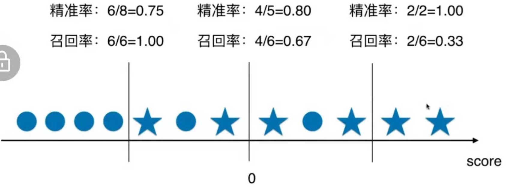
如图,图中的直线代表决策边界,决策边界右边的样本分类为1,决策边界左边的样本分类为0。图中五角星为实际类别为1的样本,0为实际类别为0的样本。
如果以0为分界点,精准率 = 4/5 = 80,召回率 = 4 / 6 = 0.67
分界点往右移,则精准率提升,召回率降低。
分界点往左移,则精准率下降,召回率提升。
用10-4中的Logic Regression对手写数字分类的例子来说明分界点移动对精准率和召回率的影响
回顾10-4的代码
准备数据
import numpy as np
from sklearn import datasets

digits = datasets.load_digits()
X = digits.data
y = digits.target.copy()

y[digits.target==9] = 1
y[digits.target!=9] = 0

from sklearn.model_selection import train_test_split
X_train, X_test, y_train, y_test = train_test_split(X, y, random_state=666)
训练模型
from sklearn.linear_model import LogisticRegression

log_reg = LogisticRegression()
log_reg.fit(X_train, y_train)
模型指标
log_reg.score(X_test, y_test)   #  0.9755555555555555

y_predict = log_reg.predict(X_test)

from sklearn.metrics import confusion_matrix
confusion_matrix(y_test, y_predict)   # array([[403,   2], [  9,  36]], dtype=int64)

from sklearn.metrics import precision_score
precision_score(y_test, y_predict)   # 0.9473684210526315

from sklearn.metrics import recall_score
recall_score(y_test, y_predict)   # 0.8

from sklearn.metrics import f1_score
f1_score(y_test, y_predict)   # 0.8674698795180723
移动Logic Regression的分界点
分析Logic Regression当前使用的分界点
上文中提到,通过调整threshold来移动决策边界,但sklearn并没有直接提供这样的接口。自带predict函数都是以0作为threshold的。
但sklearn提供了决策函数,把X_test传进去,得到的是每个样本的score值。
predict函数就是根据样本的score值来判断它的分类结果。
log_reg.decision_function(X_test)
部分输出截图:

例如前10个样本的score值是这样的,那么它们的predict结果都应该为0
log_reg.decision_function(X_test)[:10]与log_reg.predict(X_test)[:10]对比:
array([-22.05700117, -33.02940957, -16.21334087, -80.3791447 ,
-48.25125396, -24.54005629, -44.39168773, -25.04292757,
-0.97829292, -19.7174399 ])
array([0, 0, 0, 0, 0, 0, 0, 0, 0, 0])
所以可以基于decision_function来移动决策边界。
decision_scores = log_reg.decision_function(X_test)
np.min(decision_scores)   # -85.68608522646575
np.max(decision_scores)   # 19.8895858799022
移动threshold: 0->5
y_predict_2 = np.array(decision_scores >= 5, dtype='int')
confusion_matrix(y_test, y_predict_2)   # array([[404,   1], [ 21,  24]], dtype=int64)
precision_score(y_test, y_predict_2)   # 0.96
recall_score(y_test, y_predict_2)   # 0.5333333333333333
不同分界点的指标对比
| threshold | confusion_matrix | precision_score | recall_score |
|---|---|---|---|
| decision_scores >= 0(default) | array([[403, 2], [ 9, 36]], dtype=int64) | 0.9473684210526315 | 0.8 |
| decision_scores >= 5 | array([[404, 1], [ 21, 24]], dtype=int64) | 0.96 | 0.5333333333333333 |
| decision_scores >= -5 | array([[390, 15], [ 5, 40]], dtype=int64) | 0.7272727272727273 | 0.8888888888888888 |