在逻辑回归中引入了多项式，模型就会变得复杂，容易出现过拟合。
解决过拟合一个常规的手段就是在模型中添加正则化。
新的目标函数可以是：
J(theta) + a * L2或J(theta) + a * L1，其中a用于表示正则项的重要程度。
但在逻辑回归中，通常这样正则化：
C * J(theata) + L1或C * J(theata) + L2

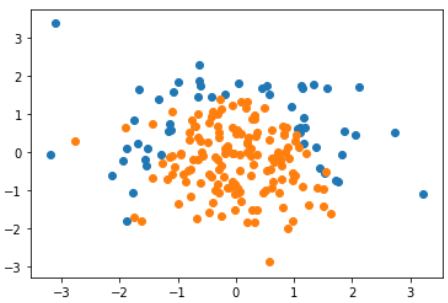
准备数据

import numpy as np
import matplotlib.pyplot as plt

np.random.seed(666)
X = np.random.normal(0, 1, size=(200,2))
y = np.array(X[:,0]**2 + X[:,1]<1.5, dtype='int')
for _ in range(20):
    y[np.random.randint(200)] = 1

plt.scatter(X[y==0,0],X[y==0,1])
plt.scatter(X[y==1,0],X[y==1,1])
plt.show()

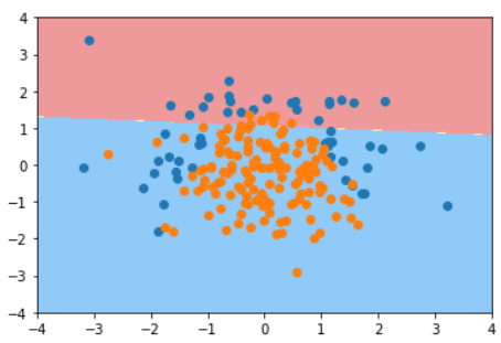
使用逻辑回归

from sklearn.linear_model import LogisticRegression

log_reg = LogisticRegression()
log_reg.fit(X_train, y_train)

log_reg.score(X_train, y_train)   # 0.79333
log_reg.score(X_test, y_test)     # 0.86

plot_decision_boundary(log_reg, [-4, 4, -4, 4])   # 使用8-6中的边界绘制算法
plt.scatter(X[y==0,0],X[y==0,1])
plt.scatter(X[y==1,0],X[y==1,1])
plt.show()

逻辑回归 + 多项式

from sklearn.pipeline import Pipeline
from sklearn.preprocessing import PolynomialFeatures
from sklearn.preprocessing import StandardScaler
from sklearn.linear_model import LogisticRegression

def PolynomialLogisticRegression(degree, C=1.0, penalty='l2'):
    return Pipeline([
        ('poly', PolynomialFeatures(degree=degree)),
        ('std_scaler', StandardScaler()),
        ('log_reg', LogisticRegression(C=C, penalty=penalty))   # 遵循sklearn标准构建的类可以无缝结合到管道中
    ])

使用不同阶数和正则化算法和C值的结果对比

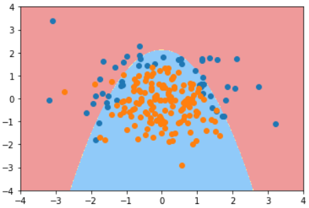
| poly_log_reg.score(X_train, y_train) | poly_log_reg.score(X_test, y_test) | plot_decision_boundary(poly_log_reg, [-4, 4, -4, 4]) --|---|---|-- degree=2 | 0.9133333333333333 | 0.94 |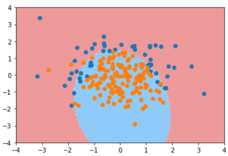
degree=20 | 0.94 | 0.92 |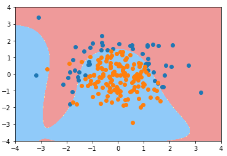
degree=20, C=0.1 | 0.8533333333333334 | 0.92(泛化能力没有降低) |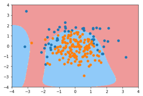
degree=20, C=0.1, penalty='l1' | 0.8266666666666667 | 0.9 |