基尼系数的计算公式： 其性质与信息熵相同。
基尼系数越大，不确定性越高。
基尼系数越小，不确定性越低。

以二分类为例，在二分类中，其中一类的概率为x，则G = -2x^2 + 2x
如果所有类别的概率相等时，基尼系数最大。类别确定时，基尼系数为0。

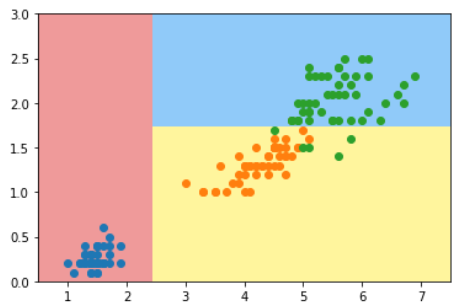
使用scikit learn中的基尼系数划分

import numpy as np
import matplotlib.pyplot as plt

from sklearn import datasets

iris = datasets.load_iris()
X = iris.data[:, 2:]
y = iris.target

from sklearn.tree import DecisionTreeClassifier

dt_clf = DecisionTreeClassifier(max_depth=2, criterion='gini')
dt_clf.fit(X, y)

def plot_decision_boundary(model, axis):
    x0, x1 = np.meshgrid(
        np.linspace(axis[0], axis[1], int((axis[1]-axis[0])*100)).reshape(-1,1),
        np.linspace(axis[2], axis[3], int((axis[3]-axis[2])*100)).reshape(-1,1)
    )
    X_new = np.c_[x0.ravel(), x1.ravel()]

    y_predict = model.predict(X_new)
    zz = y_predict.reshape(x0.shape)

    from matplotlib.colors import ListedColormap
    custom_cmap = ListedColormap(['#EF9A9A','#FFF59D','#90CAF9'])

    plt.contourf(x0, x1, zz, cmap=custom_cmap)

plot_decision_boundary(dt_clf, axis=[0.5, 7.5, 0, 3])
plt.scatter(X[y==0,0],X[y==0,1])
plt.scatter(X[y==1,0],X[y==1,1])
plt.scatter(X[y==2,0],X[y==2,1])
plt.show()

模拟使用基尼系数进行划分

代码和14-3基本上一样

from collections import Counter
from math import log

def split(X, y, d, value):
    index_a = (X[:,d] <= value)
    index_b = (X[:,d] > value)
    return X[index_a], X[index_b], y[index_a], y[index_b]

def gini(y):
    counter = Counter(y)
    res = 1.0
    for num in counter.values():
        p = num / len(y)
        res -= p ** 2
    return res

def try_split(X, y):
    best_gini = float('inf')
    best_d, best_v = -1, -1
    for d in range(X.shape[1]):
        sorted_index = np.argsort(X[:,d])
        for i in range(1, len(X)):
            if X[sorted_index[i-1], d] != X[sorted_index[i], d]:
                v = (X[sorted_index[i-1], d] + X[sorted_index[i], d]) / 2
                x_l, x_r, y_l, y_r = split(X, y, d, v)
                e = gini(y_l) + gini(y_r)
                if e < best_gini:
                    best_gini, best_d, best_v = e, d, v
    return best_gini, best_d, best_v

进行一次划分：

best_g, best_d, best_v = try_split(X, y)
print("best_g = ", best_g)
print("best_d = ", best_d)
print("best_v = ", best_v)

输出： best_g = 0.5
best_d = 0 # 代码横轴划分，表现是一根竖线
best_v = 2.45

存储划分结果：

 X1_l, X1_r, y1_l, y1_r = split(X, y, best_d, best_v)

gini(y1_l) = 0.0 # 左边只有一种数据，因此信息熵为0
gini(y1_r) = 0.5

左边已经不需要划分了，继续划分右边即可

best_g2, best_d2, best_v2 = try_split(X1_r, y1_r)
print("best_g = ", best_g2)
print("best_d = ", best_d2)
print("best_v = ", best_v2)

输出结果：
best_g = 0.2105714900645938
best_d = 1
best_v = 1.75

 X2_l, X2_r, y2_l, y2_r = split(X1_r, y1_r, best_d2, best_v2)

gini(y2_l) = 0.1680384087791495
gini(y2_r) = 0.04253308128544431

信息熵 VS 基尼系数

信息熵计算比基尼系数稍慢。
scikit-learn中默认使用基尼系数。
大多数时候二者没有特别的效果优劣。