P111
Model Adaptation
P112
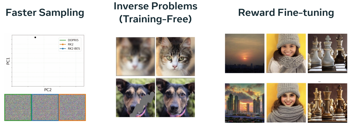
You’ve trained a model. What next?
已有一个预训练模,可以做什么?
P113
Faster Sampling
P114
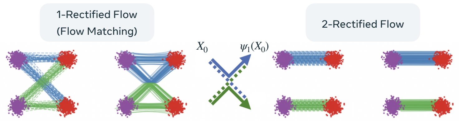
Recitde Flow-Faster sampling by straightening the flow
方法
$$ ℒ(θ) = \mathbb{E} _ {t,(X_0,X_1)∼π_ {0,1}^0}||u^θ_t (X_t) − (X_1 − X_0)||^2 $$
Rectified Flow refits using the pre-trained (noise, data) coupling.
Leads to straight flows.
Rectified Flow:让 flow 从源直接到目标。
第1步:训练 flow matching,flow matching 模型定义了源和目标的耦合关系,也得到了噪声与数据的 pair data.
第2步:用 pair data 继续训练。
🔎 “Flow Straight and Fast: Learning to Generate and Transfer Data with Rectified Flow” Liu et al. (2022)
P115
P116
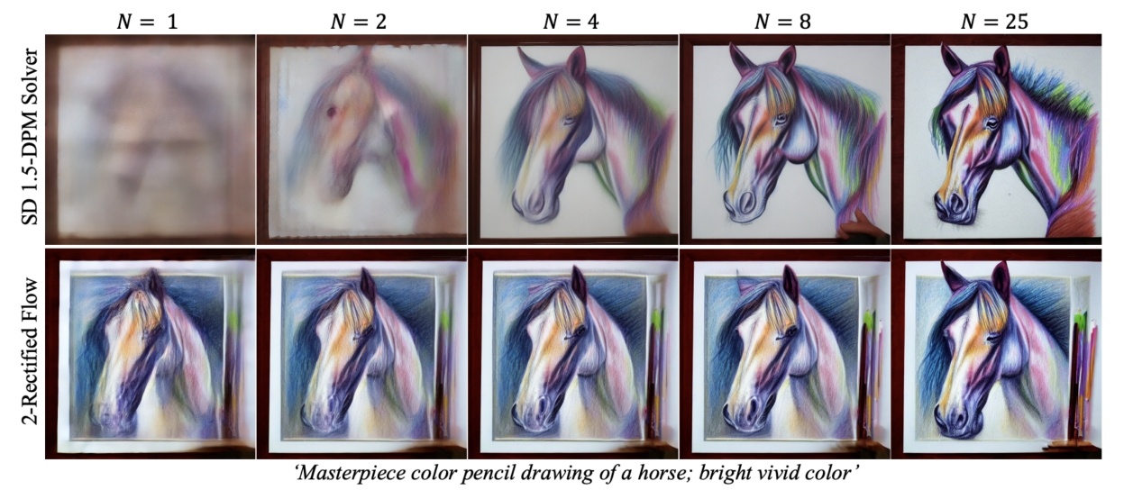
Result
Diffusion 对比 Rectified Flow
局限性
Enforcing straightness restricts the model. Often a slight drop in sample quality
🔎 “InstaFlow: One Step is Enough for High-Quality Diffusion-Based Text-to-Image Generation” Liu et al. (2022)
P118
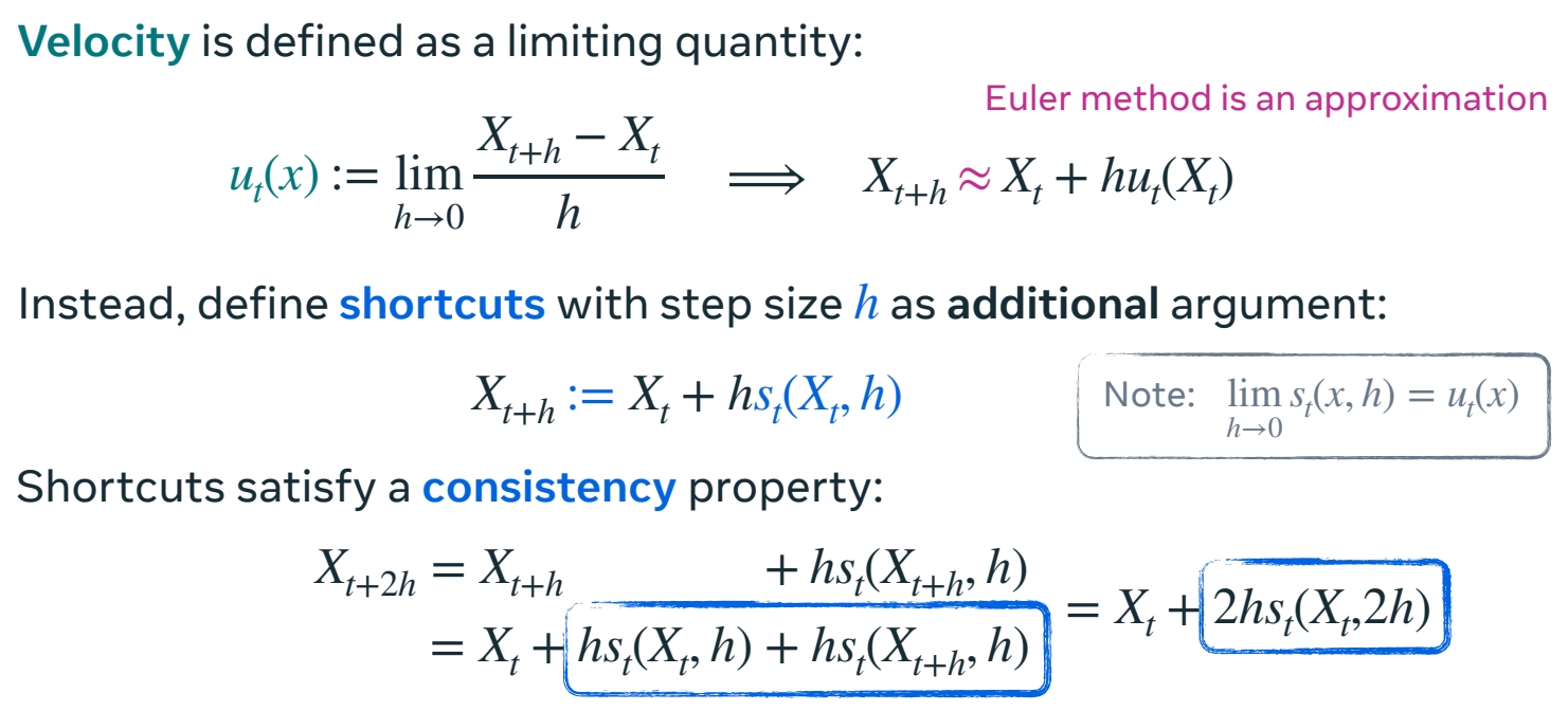
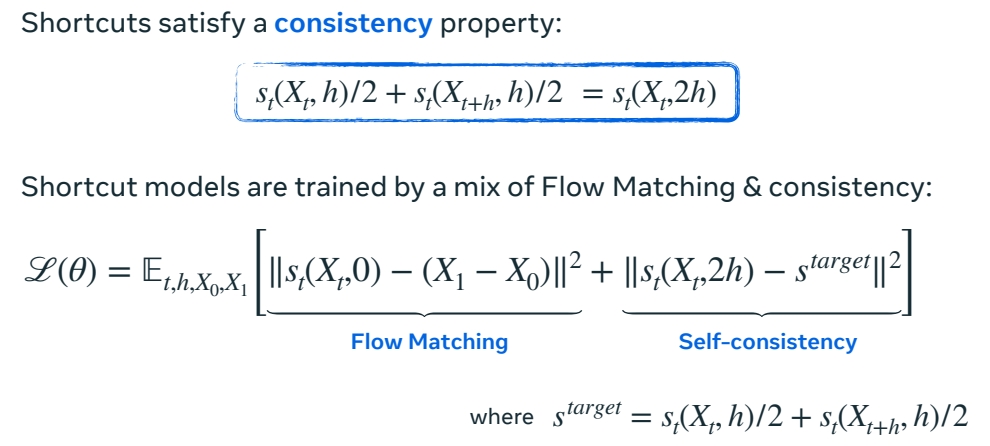
Faster sampling by self-consistency loss
增大 \(h\),在 \(x_t\) 和 \(X_{t+h}\) 之间建立 shortcut,类似于 diffusion 中的蒸馏方法。
原理
P119
方法
P121
Result
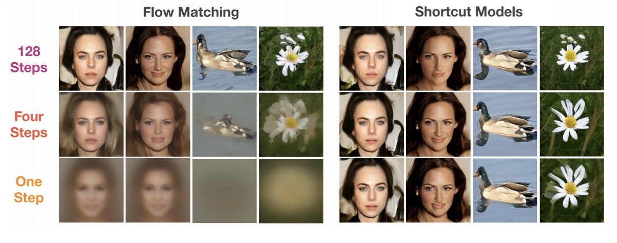
局限性
Shortcuts with \(h\) >0 do not work with classifier-free guidance (CFG).
CFG weight can & must be specified before training.
short cuts 直接预测流而不是速度,流是非线性的,不能对结果加权组合,因此不能结合 CFG.
针对此问题的 workaround:预置 CFG 权重
🔎 “One Step Diffusion via Shortcut Models” Frans et al. (2024)
P124
Faster sampling by only modifying the solver
以上两种方法,都需训练。此方法不需要训练,而是修改 solver.
补充:关于调度器.\(\beta, \alpha _t\) 和 \(\sigma _t\)的 trick.
Can adapt pre-trainedmodels to different schedulers.
有一个用 scheduler A 训练好的模型,现在要一个用 scheduler B 继续训练,这两个模型是什么关系?

结论:这两个 scheduler 及其 flow 可以通过 \(X\) 的缩放和时间的重参数化关联起来。
时间重参数化是指,匹配两个 scheduler 的 SNR 和 scaling。
Related by a scaling & time transformation:


如图所示,调整 scheduler,流会表现出不同,但 \(X_0\) 与 \(X_1\) 的耦合关系不变。
🔎 “Elucidating the design space of diffusion-based generative models” Karras et al. (2023)
P126
修改 scheduler 的例子

Bespoke solvers:
Decouples model & solver.
Model is left unchanged.
Parameterize solver and optimize.
模型与 solver 解耦:模型不变,仅优化求 solver.
向 solver 中传入参数(表达 scheduler),优化这些参数相当于在优化 scheduler。
Can be interpreted as finding best scheduler + more.
Solver consistency: sample quality is retained as NFE → ∞.
由于仅优化solver,好处:
1.可以利用 solver 的一致性,把步数取到无穷大,仍然能准确地解 ODE。做法是,用数据集 A 训练生成模型后,用数据集 B 训练 scheduler 的新参数。
2.在不同的模型(不同数据集、分辨率等训练出来的模型)之间可迁移。
Bespoke solvers can transfer across different data sets and resolutions.
局限性:
虽然能(不重训生成模型)直接迁移到另一个模型,但比在另一个模型上蒸馏(重训)效果要差一点。
P127
However, does not reach distillation performance at extremely low NFEs.
P128
相关工作
Rectified flows:
🔎 “Flow Straight and Fast: Learning to Generate and Transfer Data with Rectified Flow” Liu et al. (2022)
🔎 “InstaFlow: One Step is Enough for High-Quality Diffusion-Based Text-to-Image Generation” Liu et al. (2024)
🔎 “Improving the Training of Rectified Flows” Lee et al. (2024)
Consistency & shortcut models:
🔎 “Consistency Models” Song et al. (2023)
🔎 “Improved Techniques for Training Consistency Models” Song & Dhariwal (2023)
🔎 “One Step Diffusion via Shortcut Models” Frans et al. (2024)
Trained & bespoke solvers:
🔎 “DPM-Solver-v3: Improved Diffusion ODE Solver with Empirical Model Statistics” Zheng et al. (2023)
🔎 “Bespoke Solvers for Generative Flow Models” Shaul et al. (2023)
🔎 “Bespoke Non-Stationary Solvers for Fast Sampling of Diffusion and Flow Models” Shaul et al. (2024)
P129
Inverse Problems (Training-Free)
Inverse Problem:填充、去糊、超分、编辑。
与上节中的 data coupling 中要解决的问题不同的是,这里要利用在完全干净的数据集上训好的预训练模型,不经过重训,得到解决 Inverse Problem 的效果。
P133
Solving inverse problems by posterior inference
\(x_1\) 为干净图像,\(y\) 为噪声图像。
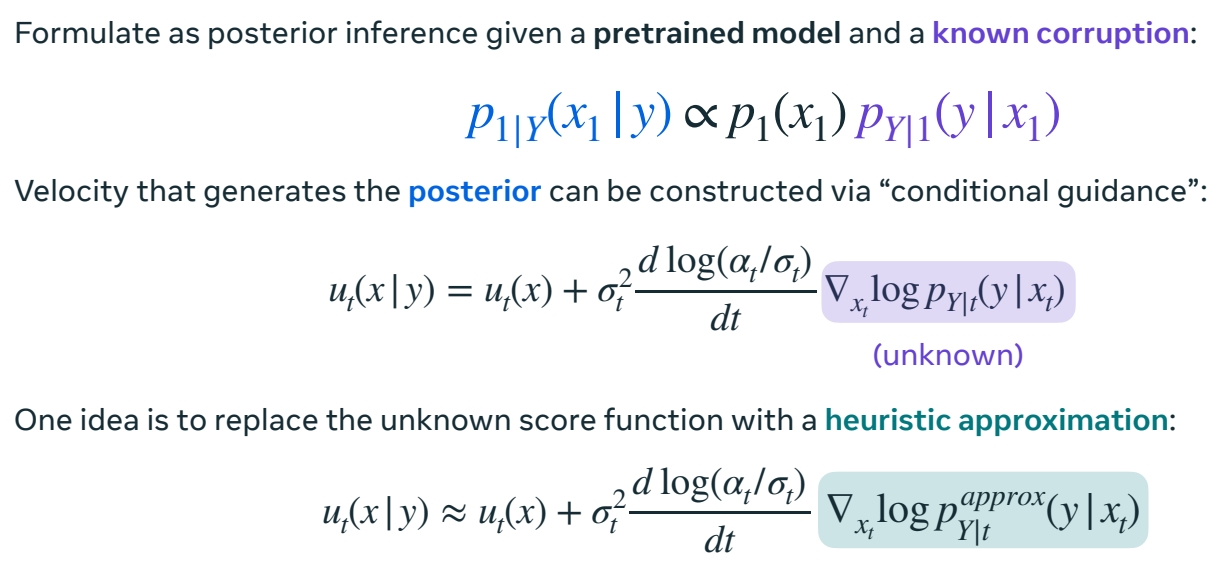
用高斯来近似其中未知的部分 (score function)
score function 可能是 multi 的,但实验证明仅用高斯也能有比较好的效果。
P134
局限性
Typically requires known linear corruption and Gaussian prob path.
Can randomly fail due to the heuristic sampling.
🔎 “Pseudoinverse-Guided Diffusion Models for Inverse Problems” Song et al. (2023)
🔎 “Training-free Linear Image Inverses via Flows” Pokle et al. (2024)
P135
Solving inverse problems by optimizing the source
观察结论
- Don’t want to rely on likelihoods / densities.
预训练一个生成模型,然后有这个模型来评估数据,评估结果很不可靠,它把数据集中的数据评估为低密度,非数据集中的数据评估为低密度。
因为,高密度\(\ne\) 高采样率。
- Have observation \(y\) being nonlinear in \(x_1\).
\(y\) 是真实图像,\(X_1\) 是模型 sample,\(X_1\) 与 \(y\) 之间差了一个 Decoder.因此它们的关系是非线性的。
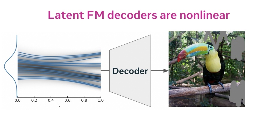
🔎 “Do Deep Generative Models Know What They Don't Know?” Nalisnick et al. (2018)
P138
方法
逆问题转化为优化问题。
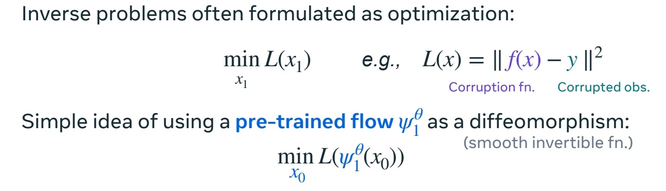
$$ X_1=\psi (X_0) $$
\(\psi \) 是预训练的生成模型,不优化 \(\psi \) 的参数,那就优化\(X_0\) 。因为 \(\psi \) 是一个平滑、可逆、可微的函数。
P139
特点与局限性
$$ \min_{x_0} L(\psi ^\theta _1(x_0)) $$
Theory: Jacobian of the flow \(\nabla _{x_0}\psi ^\theta_1\) projects the gradient along the data manifold.
Intuition: Diffeomorphism enables mode hopping!
P140
Simplicity allows application in multiple domains.
Caveat: Requires multiple simulations and differentiation of \(\psi ^\theta _1\).
求导链路很长,计算成本很高。
🔎 “D-Flow: Differentiating through Flows for Controlled Generation” Ben-Hamu et al. (2024)
P141
Inverse problems references
Online sampling methods inspired by posterior inference:
🔎 “Diffusion Posterior Sampling for General Noisy Inverse Problems” Chung et al. (2022)
🔎 “A Variational Perspective on Solving Inverse Problems with Diffusion Models” Mardani et al. (2023)
🔎 “Pseudoinverse-Guided Diffusion Models for Inverse Problems” Song et al. (2023)
🔎 “Training-free Linear Image Inverses via Flows” Pokle et al. (2023)
🔎 “Practical and Asymptotically Exact Conditional Sampling in Diffusion Models” Wu et al. (2023)
🔎 “Monte Carlo guided Diffusion for Bayesian linear inverse problems” Cardoso et al. (2023)
Source point optimization:
🔎 “Differentiable Gaussianization Layers for Inverse Problems Regularized by Deep Generative Models" Li (2021)
🔎 “End-to-End Diffusion Latent Optimization Improves Classifier Guidance” Wallace et al. (2023)
🔎 “D-Flow: Differentiating through Flows for Controlled Generation” Ben-Hamu et al. (2024)
方法 1:通过修改 sample 方法来逐步接近目标。这些方法大多数受到某种后验推断的启发,可以在准确性和效率之间 trade off.
方法 2:简单但开销很大。
P144
Reward Fine-tuning
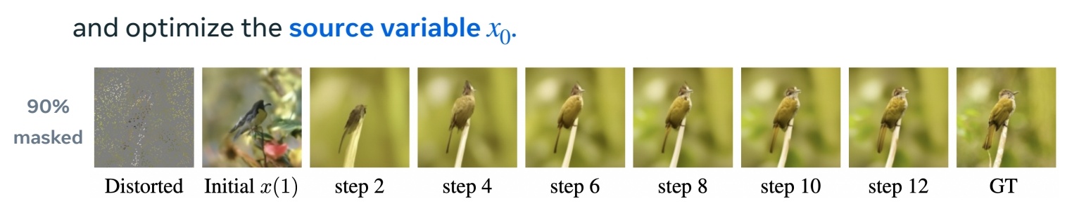
Data-driven and reward-driven fine-tuning
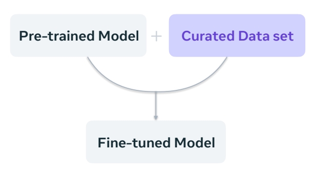 | 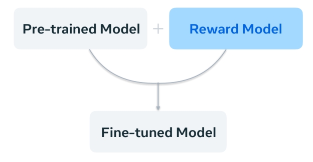 |
| A lot of focus put into data set curation through human filtering. | Can use human preference models or text-to-image alignment. |
Data-driven 的关键在于精心准备数据集。
Reward-driven 不增加训练数据,而是给模型输出一个 reward。finetune 的目标是生成得分高的 sample.
此处仅介绍后者。
P145
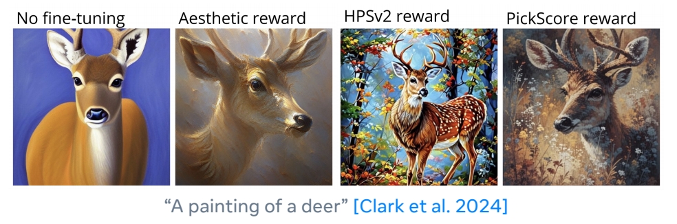
Reward fine-tuning by gradient descent
Initializing with a pre-trained flow model \(p^\theta\):
$$ \max_{\theta } \mathbb{E} _{X_1\sim p^\theta }[r(X_1)] $$
Optimize the reward model with RL [Black et al. 2023]
or direct gradients [Xu et al. 2023, Clark et al. 2024]
P146
优点:
不同的奖励模型可以组合,得到综合的效果。
局限性:
Requires using LoRA to heuristically stay close to the original model.
Still relatively easy to over-optimize reward models; “reward hacking”.
这种方法没有 GT,所以生成结果有可能对 reward model 过拟合。因此需要使用 LoRA.
🔎 “Training diffusion models with reinforcement learning” Black et al. (2023)
🔎 “Imagereward: Learning and evaluating human preferences for text-to-image generation.” Xu et al. (2023)
🔎 “Directly fine-tuning diffusion models on differentiable rewards.” Clark et al. (2024)
P149
Reward fine-tuning by stochastic optimal control
方法1:RLHF
和直接优化相比,RLHF 将一个预训练分布倾科为能得到更高奖励的分布。
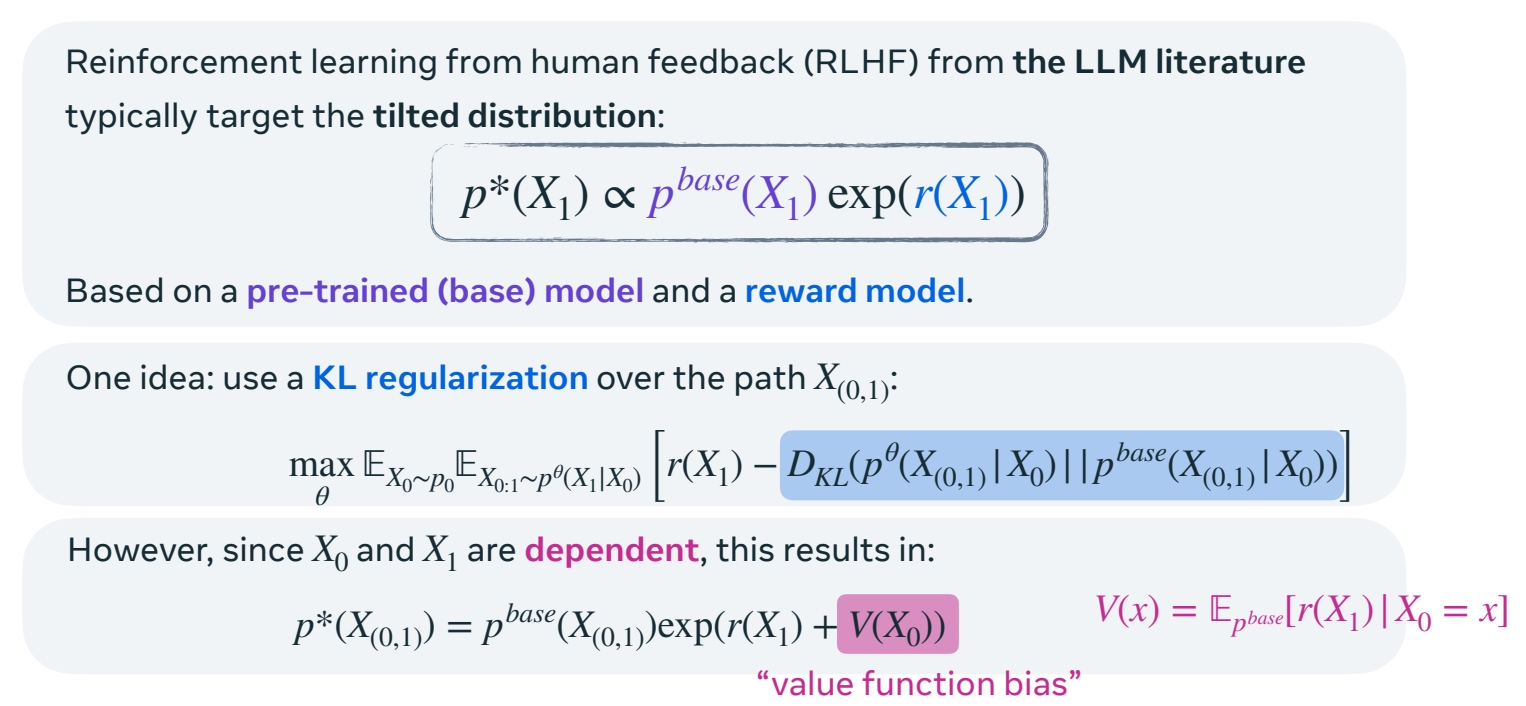
正则化:微调模型分布应与预训练模型分布接近。常用方法是增加KL 项,如下面公式蓝色部分。但这里不这样用。因为,我们要优化的不是概率路径,而是与 \(X_0\) 相关的 something.
这里采用公式(3),即引入 value function bias.
value function bias 是 \(X=X_0\)时,所有可能的 \(X_1\) 的期望。
P150
原理:
Intuition: Both initial noise \(p(X_0)\) and the model \(u_t^{base}\) affect \(p^{base}(X_1)\).
原理:某一时刻的分布受到 noise 分布和模型的共同影响,即使是同一个预预训练模型改变 noise 的分布,那么 \(X_1\) 的分布也会改变。
由于 \(X_1\) 同时受模型和 noise 分布的影响,那么 RLHF 同时优化这两个因素。
[Uehara et al. 2024] (即 RLHF) proposes to learn the optimal source distribution \(p^\ast (X_0)\).
方法2:Adjoint Matching
或者,改变采样方法,让 \(X_0\) 分布与 \(X_1\) 分布独立。那么此时,value function 是一个常数。
[Domingo-Enrich et al. 2024] proposes to remove the dependency between \(X_0, X_1\).
$$ p^\ast (X_{(0,1)})=p^{base}(X_{(0,1)})\mathrm{exp} (r(X_1)+const.)\Rightarrow p^\ast (X_1)\propto p^{base}(X_1)\mathrm{exp} (r(X_1)) $$
🔎 “Fine-tuning of continuous-time diffusion models as entropy regularized control” Uehara et al. (2024)
P151

🔎 “Adjoint matching: Fine-tuning flow and diffusion generative models with memoryless stochastic optimal control” Domingo-Enrich et al. (2024)
这篇论文的主要内容:
1.使用 flow matching 在真实图像上训练后,再使用 ODE 采样,能得到真实的输出。
2.把 ODE 过程改成无记忆 SDE(强制 \(X_0\) 与 \(X_1\) 独立),那么在早期的 sample step 实际上没有什么收益,因为那时候 \(X\) 大部分都是噪声。因此 SD 的采样结果不符合预训练的分布。
3.把 2 用于 finetune 的过程,因此 finetune 过程,不使用 flow 的 sample 方式,而是 SDE 的 sample 方式。
4.finetune 之后,可以把 SDE 换回成 ODE。
P152
Reward fine-tuning 总结
Gradient-based optimization:
🔎 “DPOK: Reinforcement Learning for Fine-tuning Text-to-Image Diffusion Models” Fan et al. (2023)
🔎 “Training diffusion models with reinforcement learning” Black et al. (2023)
🔎 “Imagereward: Learning and evaluating human preferences for text-to-image generation.” Xu et al. (2023)
🔎 “Directly fine-tuning diffusion models on differentiable rewards.” Clark et al. (2024)
Stochastic optimal control:
🔎 “Fine-tuning of continuous-time diffusion models as entropy regularized control” Uehara et al. (2024)
🔎 “Adjoint matching: Fine-tuning flow and diffusion generative models with memoryless stochastic optimal control”
Domingo-Enrich et al. (2024)
本文出自CaterpillarStudyGroup,转载请注明出处。
https://caterpillarstudygroup.github.io/ImportantArticles/