P85
Optimal Control \(\Leftrightarrow \) Reinforcement Learning
• RL shares roughly the same overall goal with Optimal Control
$$ \max \sum_{t=0}^{} r (s_t,a_t) $$
✅ 相同点:目标函数相同,是每一时刻的代价函数之和。
• But RL typically does not assume perfect knowledge of system
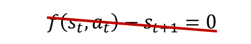
✅ 最优控制要求有精确的运动方程,而 RL 不需要。
- RL can still take advantage of a system model → model-based RL
- The model can be learned from data
$$ s_{t+1}=f(s_t,a_t;\theta ) $$
- The model can be learned from data
✅ RL 通过不断与世界交互进行采样。
P87
Markov Decision Process (MDP)
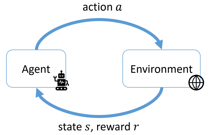
| State | \(\quad s_t \quad \quad \) |
| Action | \(\quad a_t\) |
| Policy | \(\quad \quad a_t\sim \pi (\cdot \mid s_t)\) |
| Transition probability | \(\quad \quad s_{t+1}\sim p (\cdot \mid s_t,a_t)\) |
| Reward | \(\quad \quad r_t=r (s_t,a_t)\) |
| Return | \(R = \sum _{t}^{} \gamma ^t r (s_t,a_t)\) |
✅ 真实场景中轨迹无限长,会导到 \(R\) 无限大。
✅ 因此会使用小于 1 的 \(r,t\) 越大则对结果的影响越小。
P88
跟踪问题(轨迹优化问题)变成MDP问题
用 RL 实现跟踪控制的效果
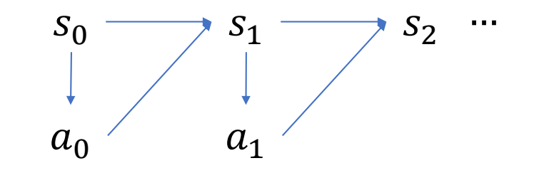
Trajectory
$$ \begin{matrix} \tau =& s_0 & a_0 & s_1 & a_1 & s_2&\dots \end{matrix} $$
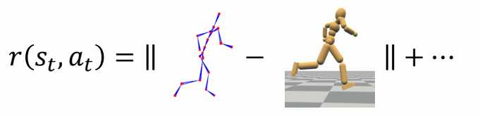
Reward
P90
MDP问题的数学描述
✅ Markov 性质:当前状态已知的情况下,下一时刻状态只与当前状态相关,而不与之前任一时刻状态相关。
MDP is a discrete-time stochastic control process.
It provides a mathematical framework for modeling decision making in situations
where outcomes are partly random and partly under the control of a decision maker.
A MDP problem:
\(\mathcal{M}\) = {\(S,A,p,r\)}
\(S\): state space
\(A\): action space
p:状态转移概率,即运动学方程。
r:代价函数。
P91
Solve for a policy \(\pi (a\mid s)\) that optimize the expected return
✅ 假设 \(\pi \) 函数和 \(p\) 函数都是有噪音的,即得到的结果不是确定值,而是以一定概率得到某个结果(期望值)。这是与最优控制问题的区别。
$$ J=E[R]=E_{\tau \sim \pi }[\sum_{t}^{} \gamma ^tr(s_t,a_t)] $$
✅ 求解一个policy \(\pi \) 使期望最优,而不是直接找最优解。
Overall all trajectories \(\tau \) = { \(s_0, a_0 , s_1 , a_1 , \dots \)} induced by \(\pi \)
P93
Bellman Equations
In optimal control:
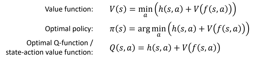
✅ 在最优控制问题中,\(\pi \) 是一个特定的策略,特指最优策略。\(V\) 也是特指在最优策略下的 value。
In RL control:

✅ 在RL控制问题中,不存在最优策略下,\(\pi \)是一个策略分布中的某一个策略,而不是最优策略。 \(V\) 是指某个策略 \(\pi \)下的 value function。
P94
How to Solve MDP
Value-based Methods
- Learning the value function/Q-function using the Bellman equations
- Evaluation the policy as
$$ \pi (s) = \arg \min_{a} Q(s,a) $$
- Typically used for discrete problems
- Example: Value iteration, Q-l a ning, DQN, …
P95
🔎 DQN [Mnih et al. 2015, Human-level control through deep reinforcement learning]
DQN 方法要求控制空间必须是离散的。但状态空间可以是离散的。
P96
相关工作
🔎 [Liu et al. 2017: Learning to Schedule Control Fragments ]
✅ DQN 方法要求控制空间必须是离散的,但状态空间可以是连续的。
✅ 因此可用于高阶的控制。
P97
Policy Gradient approach
-
Learning the value function/Q-function using the Bellman equations
-
Compute approximate policy gradient according to value functions using Monte-Carlo method
-
Update the policy using policy gradient
-
Suitable for continuous problems
-
Exa pl : REINFORCE, TRPO, PPO, …
✅ policy gradient 是 Value function 对状态参数的求导。但这个没法算,所以用统计的方法得到近似。
✅ 特点是显示定义 Policy 函数。对连续问题更有效。
P98
相关工作
 |  |  |
| [Liu et al. 2016. ControlGraphs] | [Liu et al. 2018] | [Peng et al. 2018. DeepMimic] |
P100
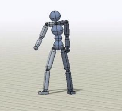
Generative Control Policies
✅ 使用RL learning,加上一点点轨迹优化的控制,就可以实现非常复杂的动作。
🔎 [Yao et al. Control VAE]
本文出自CaterpillarStudyGroup,转载请注明出处。
https://caterpillarstudygroup.github.io/GAMES105_mdbook/