P3
PD Control for Characters
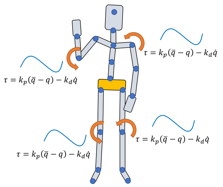
✅ 前面是 PD 的例子,这里是 PD 在物理仿真角色上的应用,计算在每个关节上施加多少力矩。
控制系统层次:PD 控制属于底层执行控制,输入是目标关节位置 $q^$ 和速度 $\dot{q}^$,输出是关节力矩 $\tau$。
中层策略:轨迹优化或 DeepMimic/AMP/ASE 等学习方法输出 PD 的目标 $q^*$。
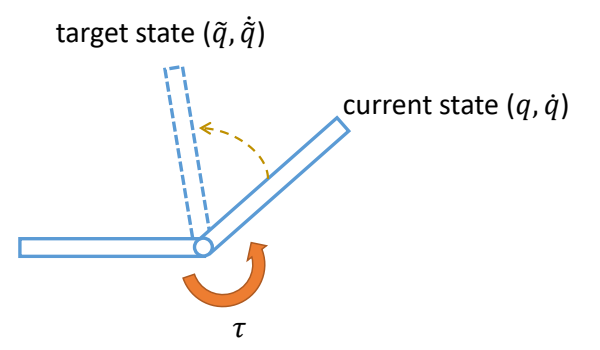
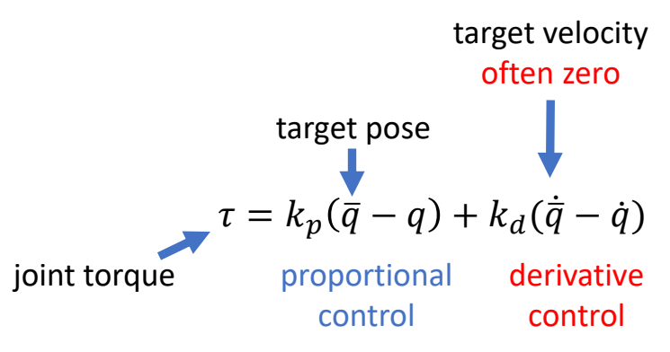
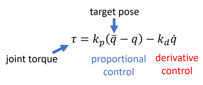
✅ 通常目标的速度 \(\dot{\bar{q}} = 0\).
因此:
P63
PD Control for Characters 的参数和效果
✅ \(K_p\) 太小:可能无法达到目标状态。 ✅ \(K_p\) 太大:人体很僵硬。 ✅ \(k_d\) 太小:动作有明显振荡。 ✅ \(k_d\) 太大,要花更多时间到达目标资态。
-
Determining gain and damping coefficients can be difficult…
- A typical setting \(k_p\) = 200, \(k_d\) = 20 for a 50kg character
- Light body requires smaller gains
- Dynamic motions need larger gains
-
High-gain/high-damping control can be unstable, so small times is necessary
- \(h\) = 0.5~1ms is often used, or 1000~2000Hz
- \(h\) = 1/120s~1/60s, or 120Hz/60Hz with Stable PD
- Higher gain/damping requires smaller time step
P66
P72
欠驱动系统问题
✅ 详细说明:参见 欠驱动系统问题
由于是欠驱动系统,Tracking Mocap with Joint Torques 会遇到问题,因为:
- \(\tau _j\): joint torques
- Apply \(\tau _j\) to "child" body
- Apply \(-\tau _j\) to "parent" body
- All forces/torques sum up to zero
✅ 合力为零,无法控制整体的位置和朝向。 ✅ 解决方法:增加净外力(Root Force/Torque),详见 欠驱动系统问题
稳态误差问题
✅ 详细说明:参见 稳态误差问题
PD control computes torques based on errors
Steady state error
This arm never reaches the target angle under gravity

在角色上的表现就是 Motion falls behind the reference
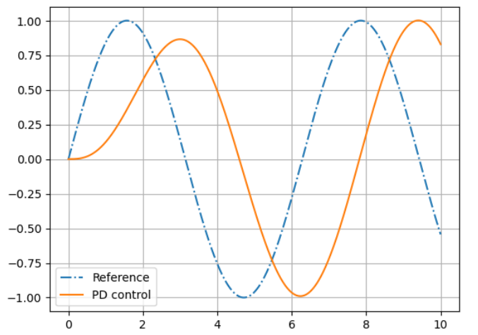
✅ 核心问题:需要有误差才能计算 force,有了 force 才能控制。 ✅ 解决方法:增大 \(k_p\)、Stable PD、前馈补偿,详见 稳态误差问题
前馈控制 vs. 反馈控制
✅ 详细说明:参见 前馈与反馈控制
Is PD control a feedforward control? a feedback control?
答案:取决于观察层次
| 观察层次 | 控制类型 | 原因 |
|---|---|---|
| 关节级别 | 反馈控制 | 使用当前关节状态 \(q\) 计算力矩 |
| 系统级别 | 前馈控制 | 目标状态由上层决定,PD 只是执行器 |
✅ 深入学习:前馈与反馈控制 - 详细讲解两者的区别、组合控制方案、以及在 DeepMimic/AMP 中的应用。
本文出自 CaterpillarStudyGroup,转载请注明出处。
https://caterpillarstudygroup.github.io/GAMES105_mdbook/