Introduction
基于LBS的3D骨骼蒙皮动画的相关技术
Refereneces
P7
3D Computer Graphics
P10
3D Computer Animation

✅ 仿真,用于描述客观事物,它们的运动规律可以用精确的数来描述。GAMES103
✅ 动画,用于描述有主观意志的事物,使用统计的方式来对它们的行为建模(例如AI建模)。 GAMES105
P11
Why Do We Study Character Animation
- A character typically has 20+ joints, or 50-100+ parameters
- It is not super high-dimensional, so most animation can be created manually, by posing the character at keyframes
- Labor-intensive, not for interactive applications
- Character animation techniques
- Understanding the mechanism behind motions and behaviors
- Smart editing of animation/ Reuse animation / Generate new animation
- “Compute-intensive”
✅ 计算机角色动画把原本劳动密集型的动画师工作变成计算密集型的工作。
P13
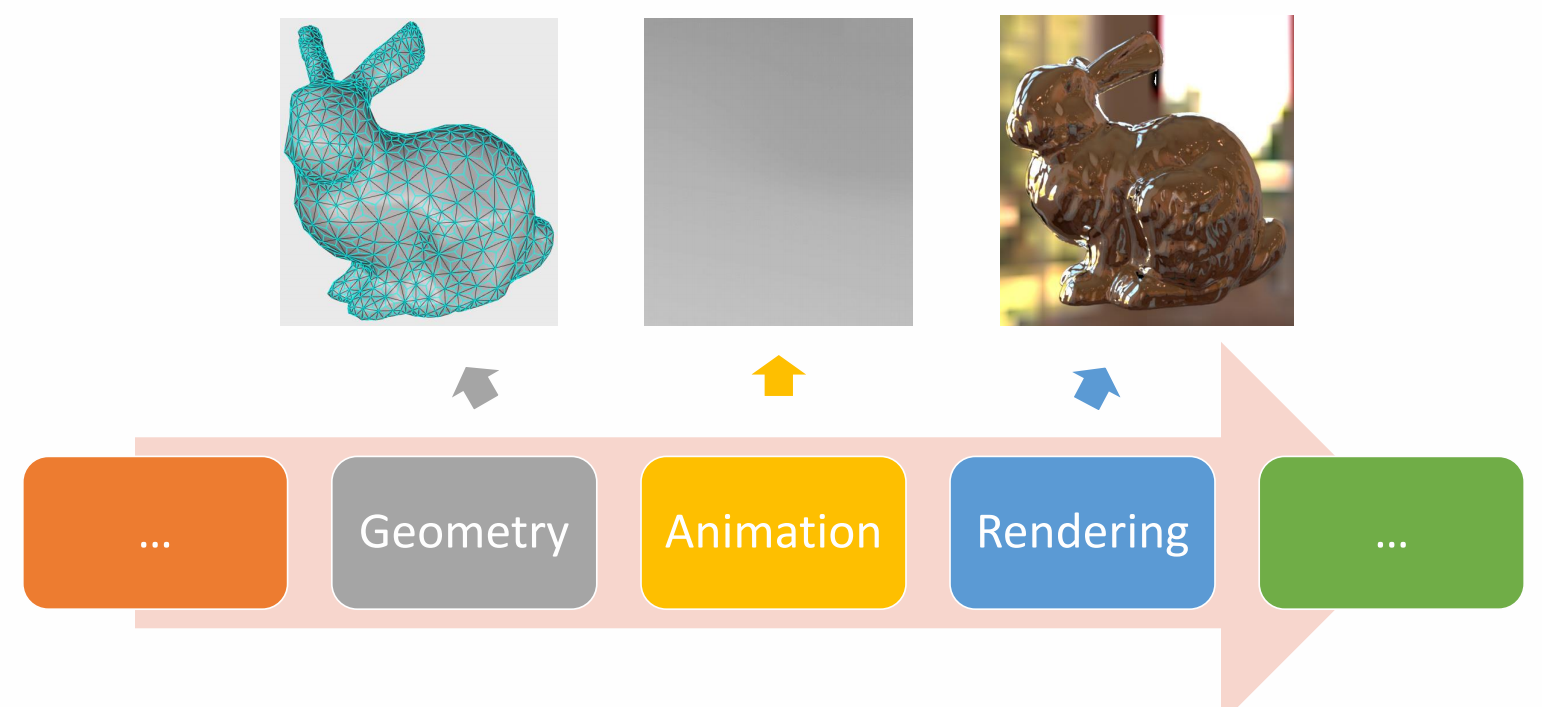
Character Animation Pipeline
P15
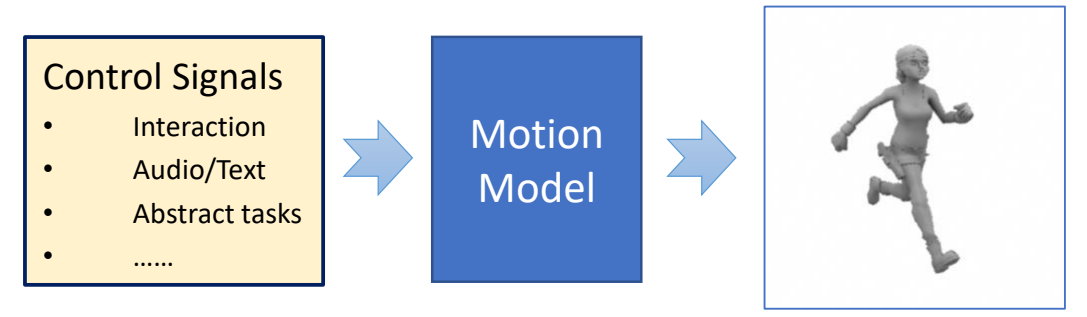
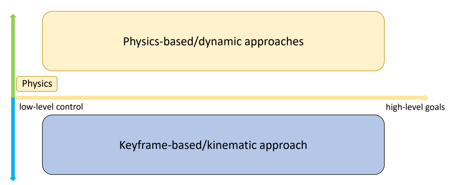
Where does a Motion Come From
根据是否使用物理,把角色动画分为两大类。
运动学 vs. 动力学对比
| 维度 | 运动学方法 (Kinematic) | 动力学方法 (Dynamic) |
|---|---|---|
| 核心思想 | 直接控制关节姿态/速度 | 通过力/力矩驱动角色 |
| 是否考虑质量 | 否 | 是 |
| 是否物理仿真 | 否 | 是 |
| 输出 | 关节姿态/速度 | 关节力矩/PD 控制目标 |
| 抗扰动能力 | 无 | 有 |
| 动作质量 | 高(来自动捕/关键帧) | 取决于控制方法 |
| 计算成本 | 低 | 高 |
| 典型应用 | 关键帧动画、Motion Matching、VR 化身 | 物理仿真、Ragdoll、交互式控制 |
✅ 运动学方法:基于运动学直接更新角色状态,运动可以不符合物理规律。 ✅ 动力学方法:基于物理仿真,但实际会有简化,不能直接干预角色姿态。
P16
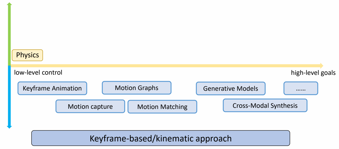
Keyframe-based/Kinematic Approaches

✅ 基于运动学直接更新角色状态,运动可以不符合物理规律。
P18
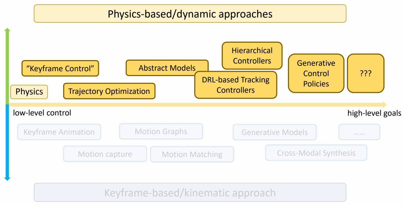
Physics-based/Dynamic Approaches
✅ 基于物理,但实际情况会有简化,不能直接干预角色姿态。
P19
Control Level
根据控制方式的高度,可以分为Low Level和Heigh Level
P20
low-level control
✅ 对每一帧每一个姿态进行精确控制每个细节。
✅ 优点:精确控制;缺点:低效。
P21
high-level control
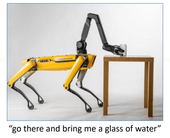
✅ 控制高级目标。
Keyframe-based/Kinematic Approaches
P24
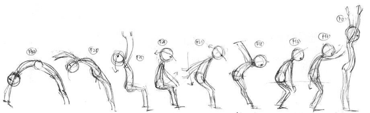
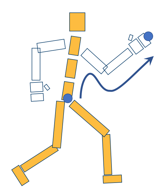
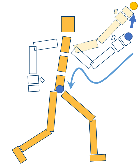
Disney’s 12 Principles of Animation
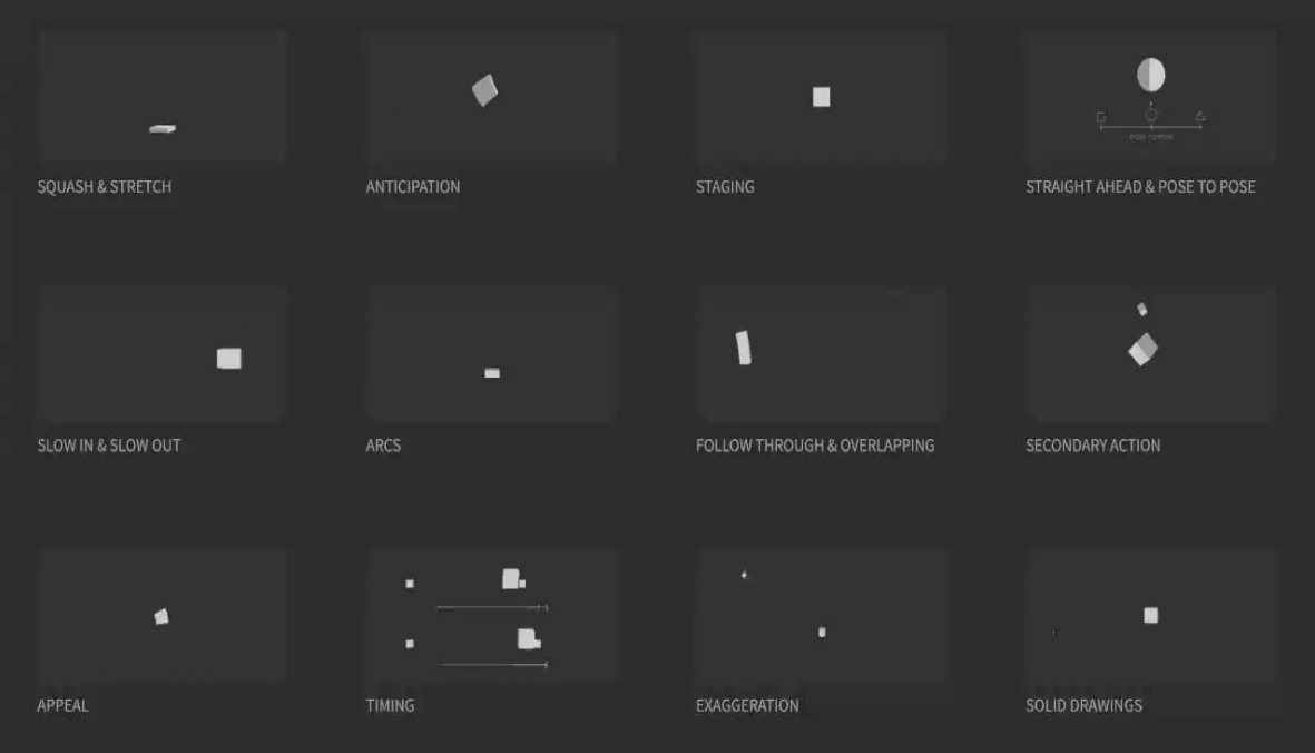
[http://the12principles.tumblr.com/]
✅ 在动画师总结的准则里隐藏了物理规则和艺术夸张
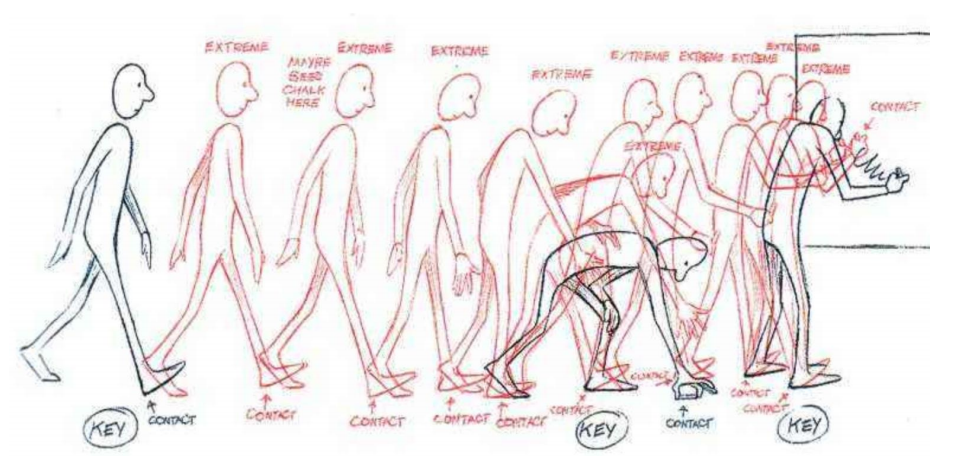
Keyframe Animation
✅ 这是一种非常low level的控制方法,可以保证所有细节,但非常慢
P26
Forward Kinematics
Given rotations of every joints
Compute position of end-effectors
P27
Inverse Kinematics
Given position of end-effectors
Compute rotations of every joints
P28
Interpolation
Motion Capture
动捕设备、视频动捕,把动捕角色应用到角色身上,需要经过重定向
动作捕捉和重放,不能产生新的数据
✅ 光学动捕、视频动捕、穿戴传感器动捕。
P34
Motion Retargeting
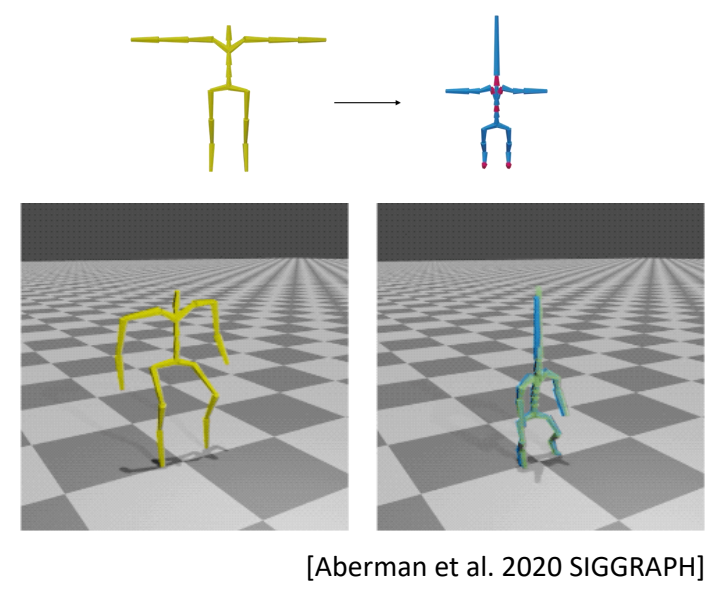
Given motions of a source character
Compute motions for target characters with
- different skeleton sizes
- different number of bones
- different topologies
- ……
P36
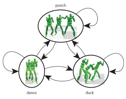
Motion Graphs / State Machines
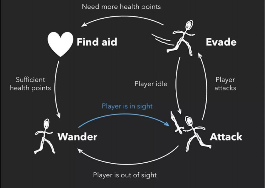
✅ 把捕出来的动作进行分解和重组,生成新的动作。
P37
Motion Graphs
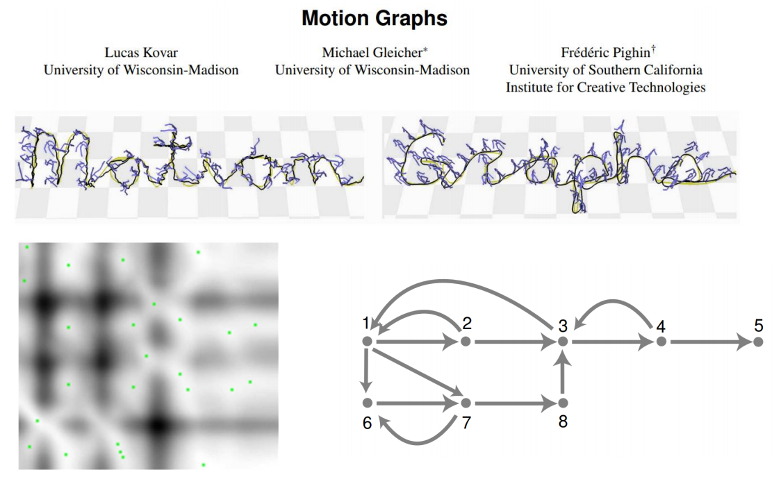
✅ 给一段任意的动作,寻找能够构建状态机切换的位。
P38
Motion Graphs的改进 - Interactively Controlled Boxing
[Heck and Gleicher 2007, Parametric Motion Graphs]
✅ 对Motion Graph的改进,比如一个节点中有很多动作,对这些动作进行插值,来实现精确控制。
P39
Motion Graphs的高级应用
Character Animation in Two-Player Adversarial Games
KEVIN WAMPLER,ERIK ANDERSEN, EVAN HERBST, YONGJOON LEE, and ZORAN POPOVIC Univoersity of Washington
Near-optimal Character Animation with Continuous Control
Adrien Treuille \(\quad\) Yongjoon Lee \(\quad\) Zoran Popovic
University of Washington
✅ Motion Graph+AI,实现高级控制
✅ 例如:AI使用Motion Graph,通过选择合适的边,进行执行,完成高级语义。
P42
Complex Motion Graphs
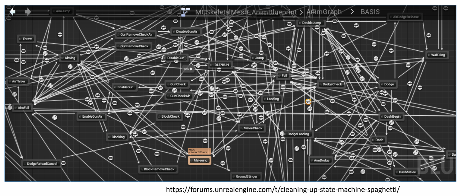
✅ 动作图非常复杂,容易出BUG.
P43
Motion Mathing
✅ 改进,Motion Graph的动作都是完整的片断,可以把动作再分细一点,切到每一帧。
✅ 不是完整地播放一段动作,而是每一帧结束后,通过最近邻搜索找到一个新的姿态,
✅ 满足:(1)接近控制目标(2)动作连续
✅ 关键:(1)定义距离函数(2)设计动作库
P45
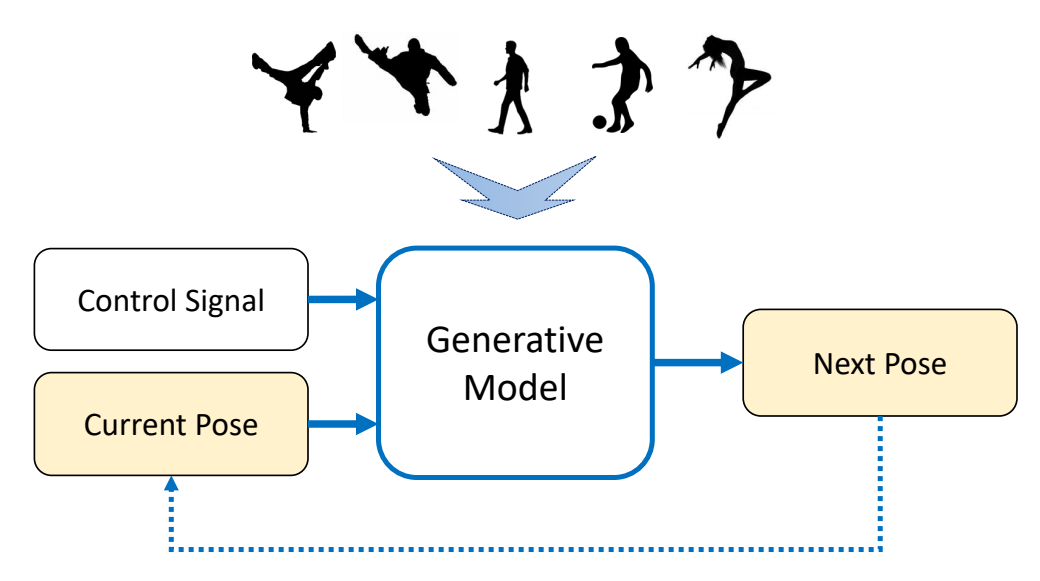
Learning-based Approaches
https://caterpillarstudygroup.github.io/ImportantArticles/CharacterAnimation/HumanMotionGenerationSummary.html
✅ 对角色动作的内在规律去理解和建模,从数据学习统计规律。
✅ 生成模型:只需要采足够的动作去给模型就能生成新的动作。
✅ 不需要手工作切分、生成状态机
P49
Cross-Modal Motion Synthesis
- Audio-driven animation
- Music to dance
- Co-speech gesture
- ……
- Natural language to animation
- Descriptions to actions
- Scripts to performance
- ……
| ID | Year | Name | Note | Tags | Link |
|---|---|---|---|---|---|
| 2022 | Rhythmic Gesticulator | ✅ 语言和动作都有内存的统计规律,把两种统计模型之间建关系,实现跨模态生成。 | 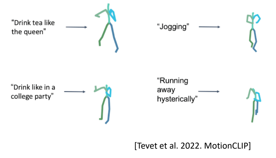 |
总结
Physics-based/Dynamic Approaches
✅ 不直接生成姿态,而是控制量(例如力),通过物理仿真真正改变角色。
P59
Ragdoll Simulation
✅ 用于人死掉、失去意识、突发事件来不及响应的情况。
P63
物理仿真角色动画的应用
[DeepMotion: Virtual Reality Tracking]
[Ye et al. 2022: Neural3Points]
[Yang et al. 2022: Learning to Use Chopsticks]
✅ 抓住手指动作细节 P67
P68
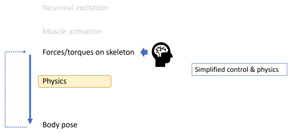
物理角色的建模方法
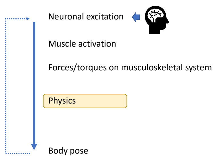
✅ 构建完整的神经系统和肌肉系统。
✅ (1)神经肌肉机理不清楚。
✅ (2)自由度高,仿真效率低。
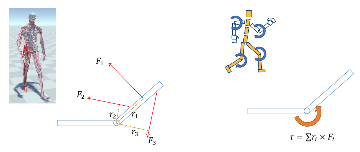
✅ 所以实际上会做简化,对关节力矩进行建模
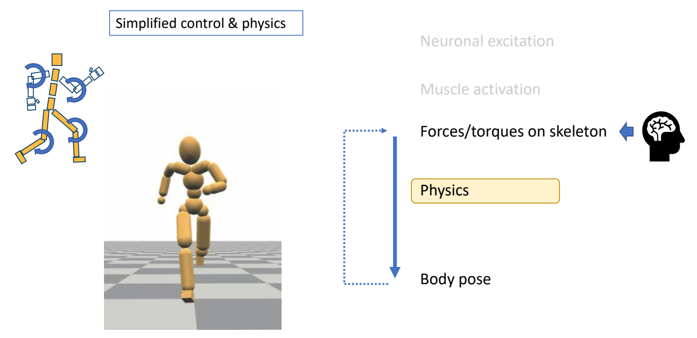
✅ 用关节力矩仿真肌肉的力。
P70
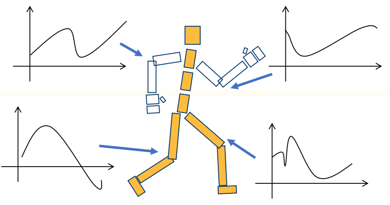
Force & Torque
P71
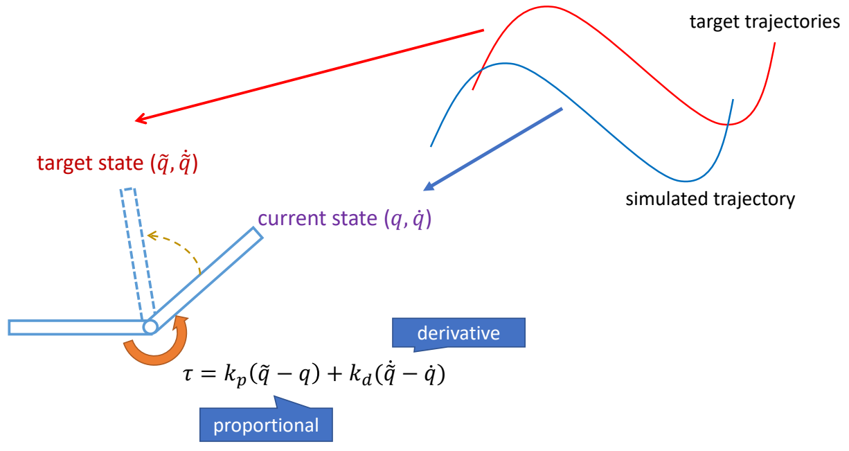
Keyfrmae Control
Proportional-Derivative (PD) Control
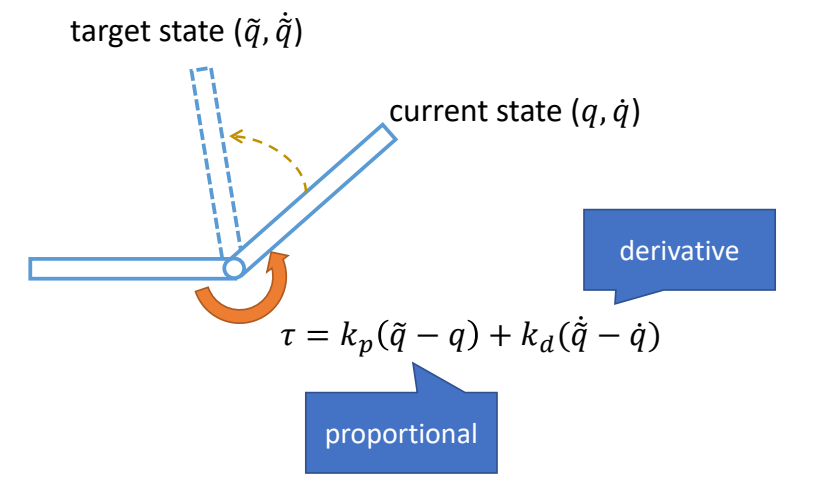
✅ 根据当前状态与目标状态的差距,计算出当前状态运动到目标状态所需要的力矩。
P72
Tracking Controllers
✅ 比如要做一个动作,给出目标高度的轨迹,采用PD控制生成每个关节的力矩,大概能产生要做的动作
[Hodgins and Wooten 1995, Animating Human Athletics]
P76
Trajectory Crafting
NaturalMotion - Endorphin
✅ 关键帧→力→仿真
实际上这个方法很难用起来,因为调整仿真参数甚至比直接做关键帧更花时间。
P79
Spacetime/Trajectory Optimization
✅ 用优化方法实现,结合重定向
[Liu et al 2010. SAMCON]
[Wampler and Popović. 2009. Optimal gait and form for animal locomotion]
[Hamalainen et al. 2020, Visualizing Movement Control Optimization Landscapes]
✅ 这是高维非线性优化问题,非常准解。
P83
Abstract Models 简化模型
通过简化模型实现对一些动作的控制,但只能做简单动作
SIMBICON
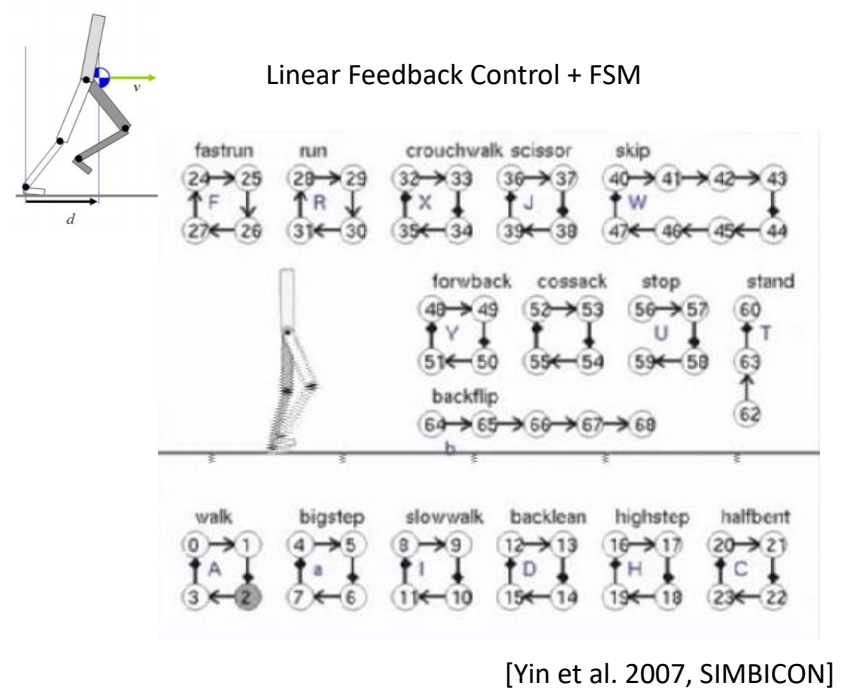
✅ 用简化模型把想要的动作描述出来,来指导角色控制。
✅ 基于此实现稳定的多技能的控制策略。
✅ 控制简化、缺少细节,走路像机器人。
✅ 简化模型思路,可以实现对一些动作进行控制,且结果鲁棒,允许使用外力与角色交互。
✅ 缺点:只能走路,不能复杂动作。
P85
Inverted Pendulum Model
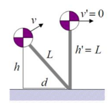
[Coros et al. 2010]
P87
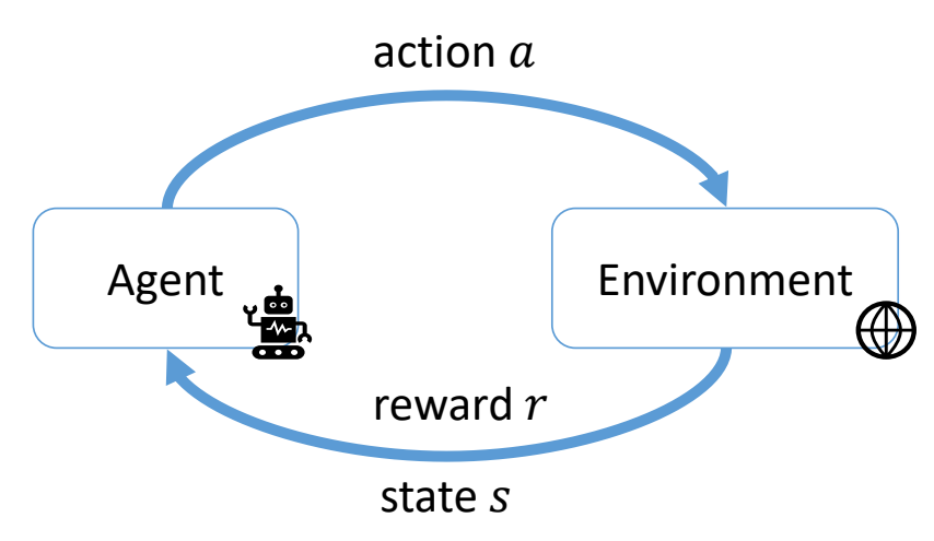
Reinforcement Learning
P89
DRL-based Tracking Controllers
[Liu et al. 2016. ControlGraphs]
[Liu et al. 2018]
[Peng et al. 2018. DeepMimic]
✅ 利用DRL做复杂动作,但还只是动作复现。
P90
Multi-skill Characters
引入状态机,完成更复杂动作。
State Machines of Tracking Controllers
引入Motion Maching
[Liu et al. 2017: Learning to Schedule Control Fragments]
Hierarchical Controllers
在高级指令控制下,综合使用动作来完成功能
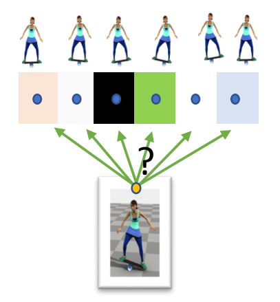
Generative Control Policies
| 运动生成模型 | 控制生成模型 |
|---|---|
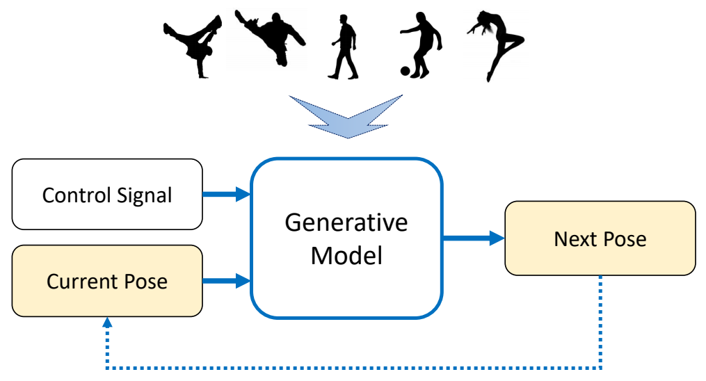 | 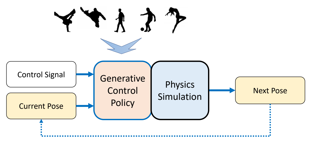 |
总结
✅ 回顾计算机角色动化领域最近30年主要研究方向。
P102
About This Course
-
What will not be covered
- How to use Maya/Motion Builder/Houdini/Unity/Unreal Engine…
- How to become an animator
-
What will be covered
-
Methods, theories, and techniques behind animation tools
- Kinematics of characters
- Physics-based simulation
- Motion control
-
Ability to create an interactive character
-
本文出自CaterpillarStudyGroup,转载请注明出处。
https://caterpillarstudygroup.github.io/GAMES105_mdbook/
P2
Outline
-
Review of Linear Algebra
- Vector and Matrix
- Translation, Rotation, and Transformation
-
Representations of 3D rotation
- Rotation matrices
- Euler angles
- Rotation vectors/Axis angles
- Quaternions
✅ 这节课大部分内容会跳过,因为前面课程讲过好多遍了
P3
Review of Linear Algebra
Vectors and Matrices
a few slides were modified from GAMES-101 and GAMES-103
P24
✅ 两个单位向量的叉乘不一定是单位向量。
✅ 要得到方向,应先叉乘再单位化
✅ \(n=\frac{a\times b}{||a\times b||}\)(正确)、\(n=\frac{a}{||a||} \times \frac{b}{||b||}\)(错误)
P26
How to find the rotation between vectors?
问题描述
✅ 已知\(a,b\) , 求旋转。
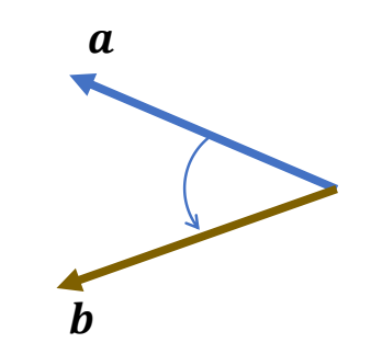
求旋转轴
P27
Any vector in the bisecting plane can be the axis
$$ 𝒖 =\frac{𝒂 × 𝒃}{||𝒂 × 𝒃||} $$
求旋转角
P28
The minimum rotation:
$$
\theta = \mathrm{arg} \cos \frac{a\cdot b}{||a||||b||}
$$
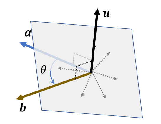
✅ \(u\) 为旋转轴,\( \theta \) 为旋转角。
P33
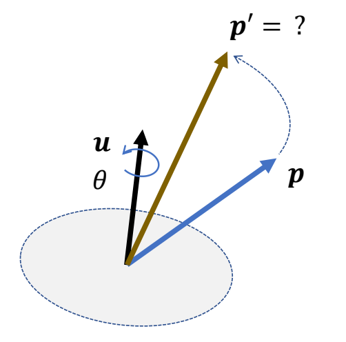
How to rotate a vectors?
问题描述
已知 \(a\) 和旋转 \((𝒖, \theta )\) 求终点 \(b\)
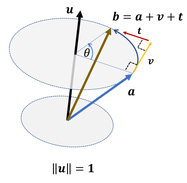
解题方法
\(a\) 移动到 \(b\) 看作是先移动 \(𝒗\) 再移动 \(t\),分别计算 \(𝒗\) 和 \(t\) 的方向和长度。
$$ 𝒗 \gets 𝒖 \times 𝒂 $$
$$ 𝒕 \gets 𝒖 \times 𝒗 = 𝒖 \times( 𝒖 \times 𝒂) $$
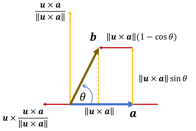
计算过程
P35
$$ 𝒗 = (\sin \theta) 𝒖 \times 𝒂 𝒕 =(1-\cos \theta ) 𝒖 \times( 𝒖 \times 𝒂) $$
Rodrigues' rotation formula
$$ 𝒃 = 𝒂 + (\sin \theta) 𝒖 × 𝒂 + (1-\cos \theta ) 𝒖 \times( 𝒖 \times 𝒂) $$
P53
Matrix
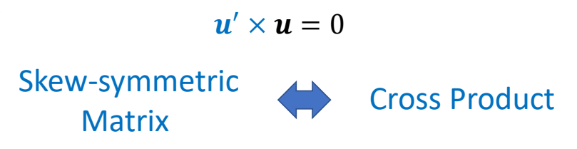
Matrix Form of Cross Product
$$ \begin{align*} c=a\times b= & \begin{bmatrix} a_yb_z-a_zb_y \\ a_zb_x-a_xb_z \\ a_xb_y-a_yb_x \end{bmatrix}\\ = & \begin{bmatrix} 0 & -a_z & a_y \\ a_z & 0 & -a_x \\ -a_y & a_x & 0 \end{bmatrix}\begin{bmatrix} b_x \\ b_y \\ b_z \end{bmatrix}=[a]_\times b \end{align*} $$
$$ [a]_\times +[a]^ \mathbf{T} _\times =0 \quad \quad \mathrm{skewsymmetric} $$
P56
$$ \begin{align*} a \times b = &[a] _ \times b \\ a \times (b \times c) = & [a] _ \times ( [b] _ \times c ) \\ = & [a] _ \times [b] _ \times c \\ a \times (a \times c) = & [a] ^2 _ \times b \\ (a \times b) \times c = & [a\times b] _ \times c \\ \end{align*} $$
✅ 最后一个公式注意一下,叉乘不满足结合律。
P57
How to rotate a vectors?
问题描述
已知 \(a\) 和旋转 \((𝒖, \theta )\) 求终点 \(b\)
把前面的结论转化为矩阵形式
$$ \begin{align*} b = & a+(\sin \theta )u \times a +(1-\cos \theta)u \times(u \times a) \\ b = & (I+(\sin \theta ))[u]_ \times + (1-(\cos \theta )[u]^2_ \times ) a \\ = & Ra \end{align*} $$
✅ 把前面的叉乘公式转化为点乘形式
结论
Rodrigues' rotation formula
$$ R = I+(\sin \theta )[u]_ \times + (1-\cos \theta )[u]^2_ \times $$
✅ \(R\) 是旋转 \((u, \theta )\) 对应的旋转矩阵。
P62
Determinant of a Matrix
定义
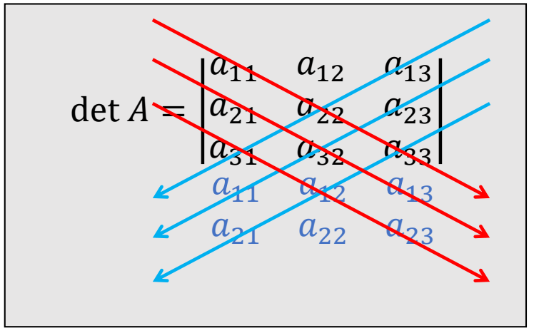
✅ 行列式的计算:红色相乘减蓝色相乘。
P63
公式
- det \(I = 1\)
- det \(AB = \text{ det } A ∗ \text{det } B\)
- det \(A^T\) = det \(A\)
- If \(A\) is invertible,det \(A^{−1}\) = \((\text{det } A)^{−1}\)
- If \(U\) is orthogonal,\(\text{det } U = ± 1\)
P64
Cross Product as a Determinant
$$ \begin{align*} c=a\times b= & \begin{bmatrix} a_yb_z-a_zb_y \\ a_zb_x-a_xb_z \\ a_xb_y-a_yb_x \end{bmatrix}\\ = & \text{det } \begin{bmatrix} i & j & k \\ a_x & a_y & a_z \\ b_x & b_y & b_z \end{bmatrix} \end{align*} $$
✅ 用行列式运算规则来计算叉乘结果。
P66
Eigenvalues and Eigenvectors
For a matrix \(A\), if a nonzero vector \(x\) satisfies
$$
Ax=\lambda x
$$
Then:
\(\lambda\): an eigenvalue of \(A\)
\(x\): an eigenvector of \(A\)
Especially, a \(3\times 3\) orthogonal matrix \(U\)
has at least one real eigenvalue: \(\lambda=\text{det } U = ±1\)
P67
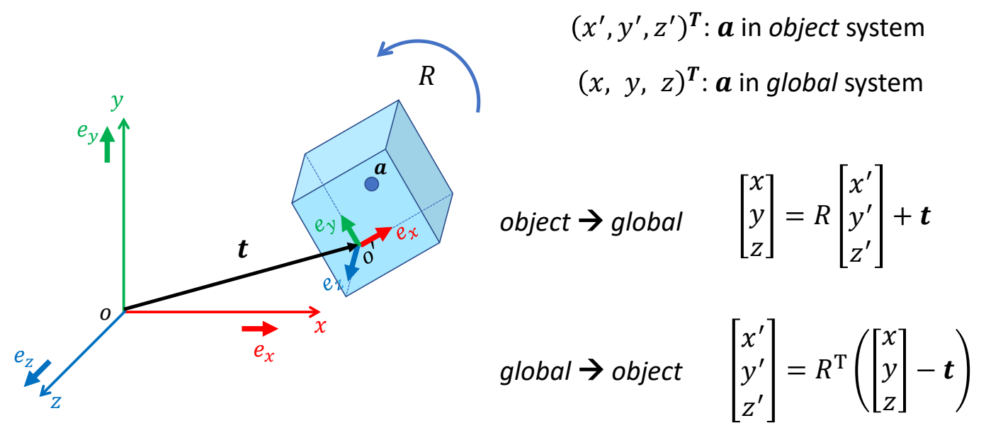
Rigid Transformation
Translation, rotation, and coordinate transformation
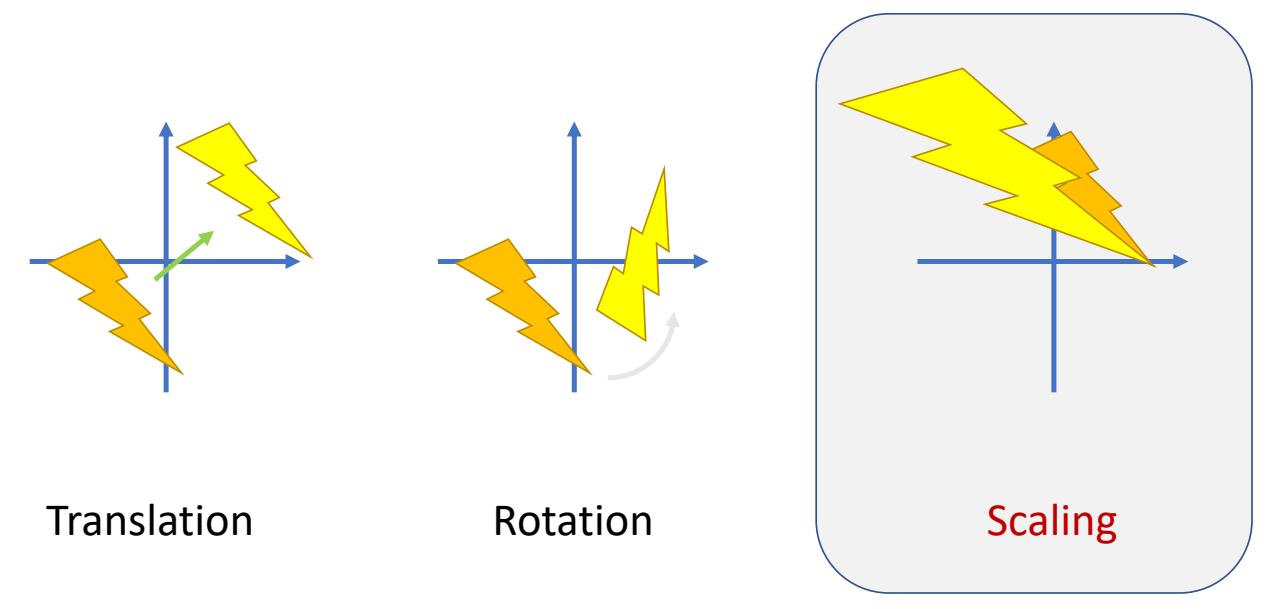
✅ 刚体变换不能改变形状和大小,因此没有Scaling
P69
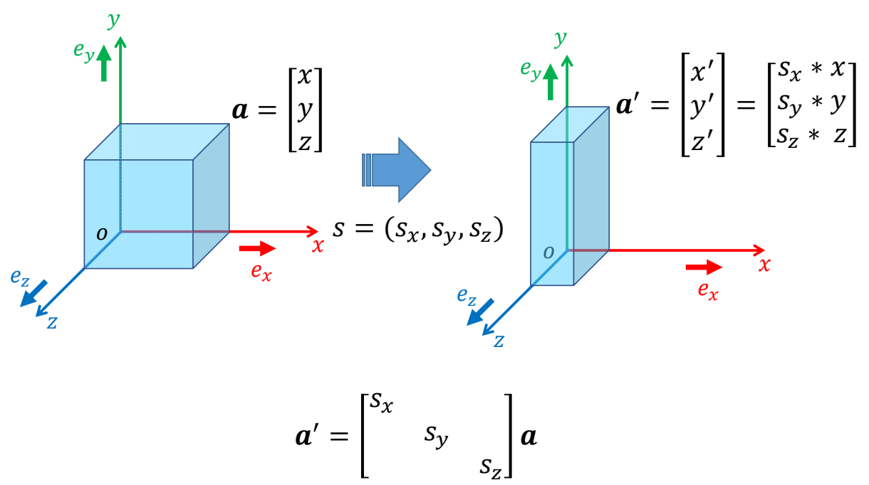
Scaling
P70
Translation

P72
Rotation

P73
Rotation Matrix
定义
- Rotation matrix is orthogonal:
$$ R^{-1}=R^{T} \quad R^TR=RR^T=1 $$
- Determinant of \(R\)
$$ \text{det } R = + 1 $$ - Rotation maintains length of vectors $$ ||Rx|| = ||x|| $$
✅ 公式2:\(R\) 不会改变左、右手系
✅ 公式3:\(R\) 是刚性变换,不改变大小
P75
Combination of Rotations

P76
Rotation around Coordinate Axes
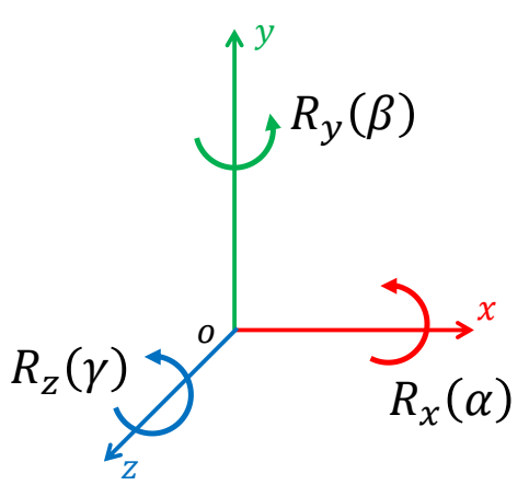
$$ R_x(\alpha )=\begin{pmatrix} 1 & 0 & 0 \\ 0 & \cos\alpha & -\sin \alpha \\ 0 & \sin \alpha & \cos \alpha \end{pmatrix} $$
$$ R_y(\beta )=\begin{pmatrix} \cos \beta & 0 & \sin \beta \\ 0 & 1 & 0 \\ -\sin \beta & 0 & \cos \beta \end{pmatrix} $$
$$ R_z(\gamma )=\begin{pmatrix} \cos \gamma & -\sin \gamma & 0 \\ \sin \gamma & \cos \gamma & 0 \\ 0 & 0 & 1 \end{pmatrix} $$
✅ 沿着哪个轴转,那个轴上的坐标不会改变。
✅ 三个基本旋转可以组合出复杂旋转。
P79
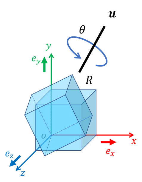
Rotation Axis and Angle
Rotation matrix \(R\) has a real eigenvalue: +1
$$
Ru=u
$$
In other words, \(R\) can be considered as a rotation around axis \(u\) by some angle \(\theta \)
How to find axis 𝒖 and angle \(\theta \)?
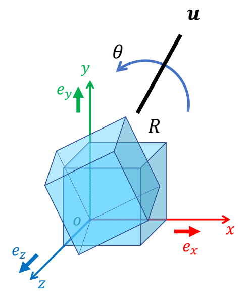
✅ 用 \(R\) 旋转时,向量 \(u\) 不会变化。
✅ 对于任意 \(R\),都存在这样一个 \(u\).
✅ \(u\) 是 \(R\) 的旋转轴。
P80
根据旋转矩阵求轴角

P81
✅ \({u}' \) 与 \({u} \) 共线,\({u}' \) 单位化得到 \({u} \).
✅ \(q\) 和 \(-q\) 两种表示方法会引入插值问题,需要注意。
P82
$$ u\gets {u}' =\begin{bmatrix} r_{32}-r_{23} \\ r_{13}-r_{31} \\ r_{21}-r_{12} \end{bmatrix} $$
$$ \text{When } R\ne R^T \Leftrightarrow \sin \theta \ne 0\Leftrightarrow \theta \ne 0^{\circ} \text{ or } 180^{\circ} $$
P83
基于罗德里格公式求轴角
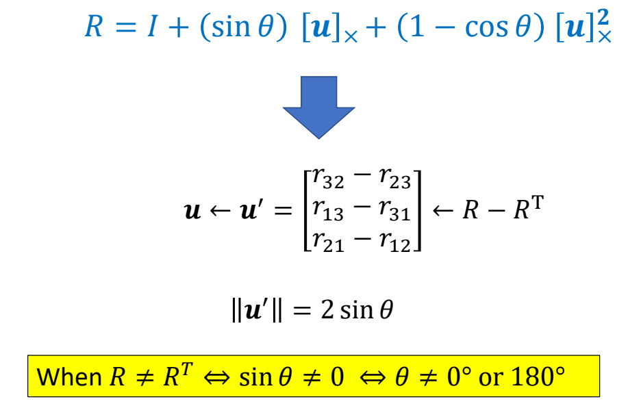
✅ 从 \(R\) 的公式也能得出相同的结论
✅ \(u → {u}' → \)旋转角度
P85
旋转矩阵的意义
旋转

P86
旋转 + 平移
P87
Representations of 3D Rotation
P91
旋转矩阵
Parameterization of Rotation
旋转矩阵有9个参数,但实际上degrees of freedom (DoF) = 3
✅ det 只是把空间减少一半,没有降低自由度
P93
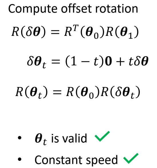
Interpolation
What is good interpolation?
- result is valid at any time \(t\)
- Constant speed is preferred
| 平移 | 旋转 | |
|---|---|---|
 | 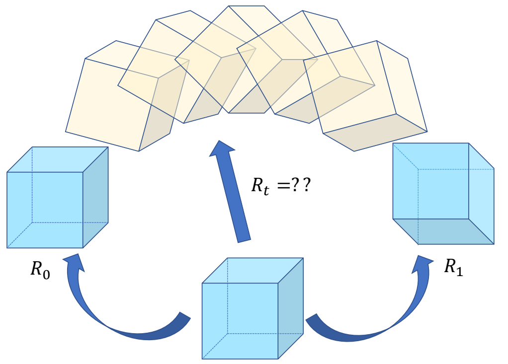 | |
| \(x_t=(1-t)x_0+tx_1\) ✅ 平移使用线性插值 | ✅ 旋转不适合线性插值。 | |
| 合法 | ✅ 对于任意 \(t\), \(x_t\) 一定是合法的。 | |
| 速度可控 | ✅ 运动的速度是常数,因此速度可控。 |
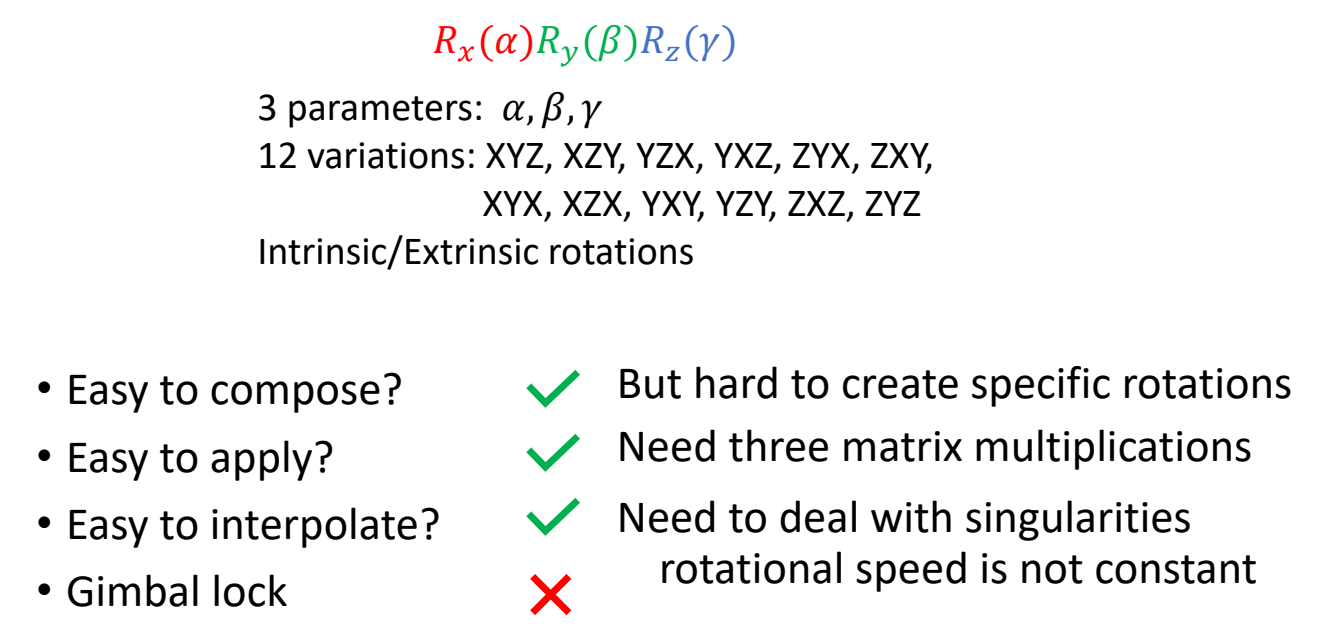
P99
结论
- Easy to compose? \(\quad \quad \quad {\color{Red} \times } \)
✅ 9个参数没有直接的意义,且为了满足正交阵,参数之间是耦合的。
- Easy to apply? \(\quad \quad \quad \quad {\color{Green} \surd }\)
- Easy to interpolate? \(\quad \quad {\color{Red} \times } \)
P100
Euler angles
Basic rotations

$$ R_x(\alpha )=\begin{pmatrix} 1 & 0 & 0 \\ 0 & \cos\alpha & -\sin \alpha \\ 0 & \sin \alpha & \cos \alpha \end{pmatrix} $$
$$ R_y(\beta )=\begin{pmatrix} \cos \beta & 0 & \sin \beta \\ 0 & 1 & 0 \\ -\sin \beta & 0 & \cos \beta \end{pmatrix} $$
$$ R_z(\gamma )=\begin{pmatrix} \cos \gamma & -\sin \gamma & 0 \\ \sin \gamma & \cos \gamma & 0 \\ 0 & 0 & 1 \end{pmatrix} $$
combination of three basic rotations
Any rotation can be represented as a combination of three basic rotations
P102
Any combination of three basic rotations are allowed
- Excluding those rotate twice around the same axis
- XYZ, XZY, YZX, YXZ, ZYX, ZXY, XYX, XZX, YXY, YZY, ZXZ, ZYZ
P103
Conventions of Euler Angles
intrinsic rotations: axes attached to the object
$$ R_x(\alpha )R_y(\beta )R_z(\gamma ) $$
extrinsic rotations: axes fixed to the world
$$ R_z(\gamma )R_y(\beta )R_x(\alpha ) $$
✅ 使用欧拉角时应先明确所使用的 convetion 和顺序。
✅ 不同的商业软件可能有不同的内置参数。
✅ maya 和 unity 都是 extrinsic.
✅ maya 可选顺序,Unity 固定 Zxy
P104
Gimbal Lock
When two local axes are driven into a parallel configuration, one degree of freedom is “locked”
✅ 当其中两个轴共线时,会丢失一个自由度,此时表示不唯一(奇异点)
P105
结论
✅ 插值时需注意作用域为 \([-\pi , \pi ]\),否则容易出现翻转现象。
P107
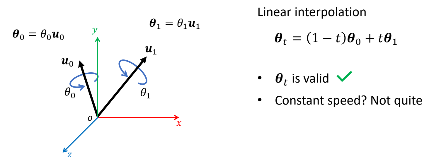
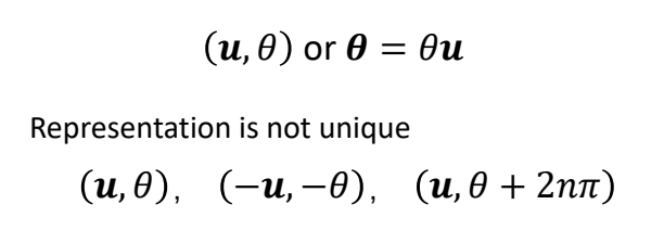
Rotation Vectors / Axis Angles

✅ 粗体 \(\theta \):轴角表示法描述的旋转
✅ 细体 \(\theta \):以 \(u\) 为轴的旋转角度
✅ 应用时要先转为旋转矩阵,做旋转组合时也要借助旋转矩阵
P110
Interpolating Rotation Vectors / Axis Angles
线性插值
可以保证插值结果合法,但不能保证旋转速度恒定
P111
匀速插值
可以保证插值结果合法且匀速,但旋转较复杂
✅ 这个方法没听懂,可以实现允许插值。
P112
结论
- Easy to compose? \(\quad \quad {\color{Green} \surd } \quad \quad \) But hard to manipulate
- Easy to apply? \(\quad \quad \quad {\color{Red} \times } \quad \quad \) Need to convert to matrix
- Easy to interpolate? \(\quad \quad {\color{Green} \surd } \quad \quad \) Linear interpolation works, but not perfect
- No Gimbal lock \(\quad \quad {\color{Green} \surd } \quad \quad \) need to deal with singularities
P113
Quaternions
P116
定义
-
Extending complex numbers
$$ q =a+bi +cj +dk \in \mathbb{H} ,a,b,c,d\in \mathbb{R} $$ -
\(i^2=j^2=k^2=ijk=-1\)
-
\(ij=k,ji=-k(^*\text{cross product})\)
-
\(jk=i,kj=-i\)
-
\(ki=j,ik=-j\)
$$ q=w+xi+yj+zk \quad \Rightarrow \quad q=\begin{bmatrix} w\\ x\\ y\\ z \end{bmatrix}=\begin{bmatrix} w\\ v \end{bmatrix} $$
$$ q =[w,v]^T \in \mathbb{H} ,w\in \mathbb{R},v\in \mathbb{R}^3 $$
$$ w =[w,0]^T : \text{ scalar quaternion } $$
$$ v =[0,v]^T : \text{ pure quaternion } $$
P117
Quaternion Arithmetic
$$ q =a+bi +cj +dk \in \mathbb{H} ,a,b,c,d\in \mathbb{R} $$
Conjugation: \(\quad \quad q^*=a-bi-cj-dk\)
\(
\)
Scalar product: \(\quad \quad tq=ta+tbi+tcj+tdk\)
\(
\)
Addition: \(\quad \quad q_1+q_2=(a_1+a_2)+(b_1+b_2)i+(c_1+c_2)j+(d_1+d_2)k\)
\(
\)
Dot product: \(\quad \quad q_1\cdot q_2=a_1a_2+b_1b_2+c_1c_2+d_1d_2\)
\(
\)
Norm: \(\quad \quad ||q||=\sqrt{a^2+b^2+c^2+d^2} =\sqrt{q\cdot q}\)
P118
Quaternion Multiplication
$$ q_1q_2=(a_1+b_1i+c_1j+d_1k)*(a_2+b_2i+c_2j+d_2k) $$
$$ q_1q_2=a_1a_2-b_1b_2-c_1c_2-d_1d_2 $$
$$
+(b_1a_2+a_1b_2-d_1c_2+c_1d_2)i
$$
$$
+(c_1a_2+d_1b_2+a_1c_2-b_1d_2)j
$$
$$ +(d_1a_2-c_1b_2+b_1c_2+a_1d_2)k $$
note:
- \(i^2=j^2=k^2=ijk=-1\)
- \(ij=k,ji=-k (^* \text{cross product})\)
- \(jk=i,kj=-i\)
- \(ki=j,ik=-j\)
✅ \(q_1 \cdot q_2\) 和 \(q_1q_2\) 是两种不同的运算。
P120
Conjugation: \(\quad \quad q^*=[w,-v]^T\)
\(
\)
Scalar product: \(\quad \quad tq=[tw,tv]^T\)
\(
\)
Addition: \(\quad \quad q_1+q_2=[w_1+w_2,v_1+v_2]^T\)
\(
\)
Dot product: \(\quad \quad q_1\cdot q_2=w_1w_2+v_1 \cdot v_2\)
\(
\)
Norm: \(\quad \quad ||q||=\sqrt{w_1w_2+v_1 \cdot v_2} =\sqrt{q\cdot q}\)
P122
$$ q_1q_2=\begin{bmatrix} w_1\\ v_1 \end{bmatrix}\begin{bmatrix} w_2 \\ v_2 \end{bmatrix}=\begin{bmatrix} w_1w_2-v_1\cdot v_2\\ w_1v_2+w_2v_1+v_1\times v_2 \end{bmatrix} $$
Non-Commutativity:
$$ q_1q_2\ne q_2q_1 $$
Associativity:
$$ q_1q_2q_3=(q_1q_2)q_3=q_1(q_2q_3) $$
P123
Conjugation:
$$ (q_1q_2)^\ast=q^\ast_2q^\ast_1 $$
Norm:
$$ ||q||^2 = q^ \ast q =qq^\ast $$
Reciprocal:
$$ \begin{matrix} qq^{-1}=1 & \Rightarrow & q^{-1}=\frac{q^*}{||q||^2}\\ q^{-1}q=1 & & \end{matrix} $$
P124
Unit Quaternions
$$ \begin{matrix} q=\begin{bmatrix} w\\ v \end{bmatrix} &||q||=1 \end{matrix} $$
For any non-zero quaternion \(\tilde{q} \):
$$ q=\frac{\tilde{q}}{||\tilde{q}||} $$
Reciprocal:
$$ \begin{matrix} q^{-1}=q^\ast =\begin{bmatrix} w\\ -v \end{bmatrix} &\Leftrightarrow & R^{-1}=R^T \end{matrix} $$
P125
| 2D | 3D |
|---|---|
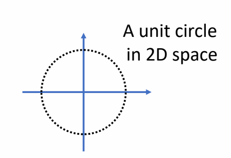 |  |
| unit complex number | unit quaternion ✅ 所有单位四元数构成 4D 空间上的单位球核。 |
| \(z = \cos \theta + i\sin \theta\) | \(q = \begin{bmatrix} w\\v\end{bmatrix}= [\cos \frac{\theta}{2} , u\sin \frac{\theta}{2}] \quad \mid\mid u \mid\mid = 1\) |
same information as axis angles \((u,\theta)\) But in a different form
P127
轴角表示 -> 四元数表示
Any 3D rotation \((v,\theta)\) can be represented as a unit quaternion
$$ \begin{matrix} \text{Angle}: & \theta =2 \text{ arg } \cos w\\ \text{ Axis}: & u=\frac{v}{||v||} \end{matrix} $$
P128
Rotation a Vector Using Unit Quaternions
已经向量p和单位四元数q,求p经过q旋转后的向量。
$$ \begin{matrix} \text{Unit quaternion}: & q=\begin{bmatrix} w\\ v \end{bmatrix}=[\cos \frac{\theta }{2} ,u\sin \frac{\theta }{2}]\\ \text{ 3D vector}:p & \text{ Rotation result }: {p}' \end{matrix} $$
Then the rotation can be applied by quaternion multiplication:
✅ 纯方向 \(p\) 可用四元数表示为 \([0 \quad p ]\)
✅ \({p}' = R (q) \cdot p\)
P129
$$ \begin{bmatrix} 0 \\ {p}' \end{bmatrix}=q\begin{bmatrix} 0\\ p \end{bmatrix}q^\ast =(-q)\begin{bmatrix} 0\\ p \end{bmatrix}(-q)^\ast $$
\(\mathbf{q}\) and \(−\mathbf{q}\) represent the same rotation
P131
Combination of Rotations
证明过程跳过,结论:
$$ \begin{matrix} \text{Combined rotation}: & q=q_2q_1 \end{matrix} $$
P133
Quaternion Interpolation
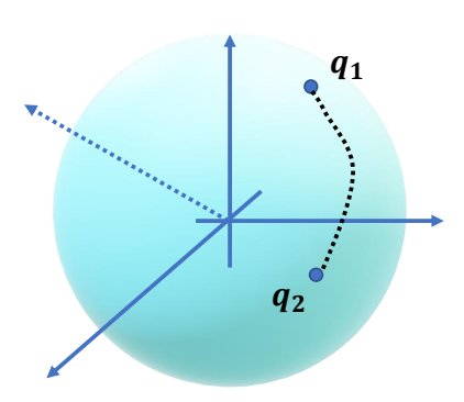
A unit hypersphere in 4D space
✅ 单位四元数表现出来是 4D 空间中的球核,\(q_1q_2\) 是球核上的两个点,希望沿球面轨迹插值。
P135
Linear Interpolation
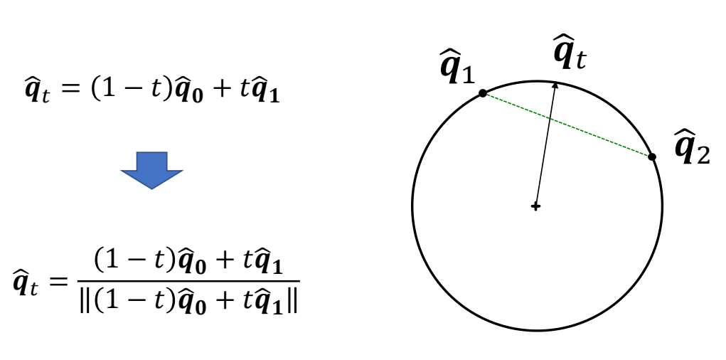
$$ q_t=(1-t)q_0+tq_1 $$
\(q_t\) is not a unit quaternion
P136
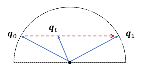
Linear Interpolation + Projection
$$ \begin{matrix} \tilde{q}_t=(1-t)q_0+tq_1 & q_t=\frac{\tilde{q}_t }{||\tilde{q}_t||} \end{matrix} $$
$$ \begin{matrix} q_t \text{ is a unit quaternion}\\ \text{Rotational speed is not constant} \end{matrix} $$
✅ 当 \(u_0=-u_1\) 时,可能得到某个 \(\tilde{q} _t = 0\),无法单位化
✅ 解决方法:根据 \(u_0=-u_0\),先找到 \(u_0\) 和 \(u_1\) 在数值上最接近的四元数表示。
P137
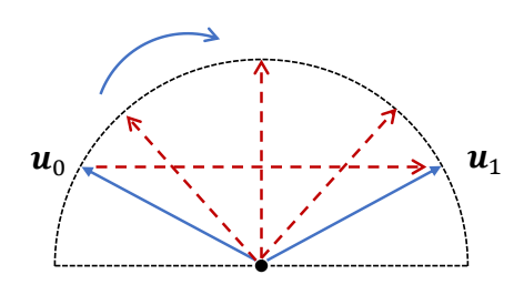
SLERP: Spherical Linear Interpolation
思考
$$ q_t=a(t)q_0+b(t)q_1 $$
如何设计a和b,让插值结果速度恒定?

$$ r=a(t)p+b(t)q $$
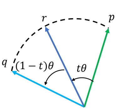
计算
Consider the angle \(\theta\) between \(p,q\):
$$ \cos \theta =p\cdot q $$
We have:
$$ \begin{matrix} p \cdot r=a(t)p\cdot p+b(t)q\cdot p\\ \Rightarrow \cos t \theta =a(t)+b(t)\cos \theta \end{matrix} $$
similarly:
$$
\begin{matrix}
q \cdot r=a(t)q\cdot p+b(t)\\
\Rightarrow \cos (1- t) \theta =a(t)\cos\theta +b(t)
\end{matrix}
$$
结论
then we have:
$$ a(t)=\frac{\sin [(1-t)\theta ]}{\sin \theta } ,b(t)=\frac{\sin t \theta }{\sin \theta } $$
P139
$$ q_t=\frac{\sin [(1-t)\theta ]}{\sin \theta }q_0+\frac{\sin t \theta }{\sin \theta }q_1 $$
$$ \cos \theta=q_0\cdot q_1 $$
P140
结论
Rotations can be represented by unit quaternions
Representation is not unique
\(q, −q\) represent the same rotation
- Easy to compose? \(\quad \quad {\color{Green} \surd }\quad \quad \) Need normalization, hard to manipulate,
- Easy to apply? \(\quad \quad \quad {\color{Green} \surd }\quad \quad \) Quaternion multiplication
- Easy to interpolate? \(\quad {\color{Green} \surd }\quad \quad \) SLERP, need to deal with singularities
- No Gimbal lock \(\quad \quad \quad {\color{Green} \surd }\quad \quad \)
本文出自CaterpillarStudyGroup,转载请注明出处。
https://caterpillarstudygroup.github.io/GAMES105_mdbook/
角色位移控制 (Locomotion Control) 技术洞察
更新时间: 2026-03-30
范围: 2010-2025 年角色位移 (locomotion) 控制技术分析
一、概述
角色位移控制是计算机图形学、机器人学和游戏开发的核心问题,目标是生成自然、稳定、可控的角色运动(如行走、跑步、跳跃等)。
1.1 为什么 Locomotion 是一个难题?
- 高维状态空间: 人形角色通常有 30+ 自由度
- 强非线性动力学: 接触力、摩擦力、碰撞使系统高度非线性
- 多模态行为: 行走、跑步、跳跃等不同步态需要不同控制策略
- 实时性要求: 游戏/VR 应用需要 60+ FPS
- 鲁棒性要求: 需要抵抗外部扰动、适应地形变化
1.2 技术分类:运动学 vs 动力学
| 维度 | 运动学方法 (Kinematics) | 动力学方法 (Dynamics) |
|---|---|---|
| 核心目标 | 生成视觉上合理的动作 | 生成物理可行的动作 |
| 输出 | 关节姿态/速度 | 关节力矩/PD 控制目标 |
| 是否物理仿真 | 否 | 是 |
| 典型应用 | 动画生成、VR 化身 | 游戏、机器人仿真 |
| 优势 | 速度快、质量高 | 物理交互、抗扰动 |
| 局限 | 无法处理物理交互 | 训练成本高、实现复杂 |
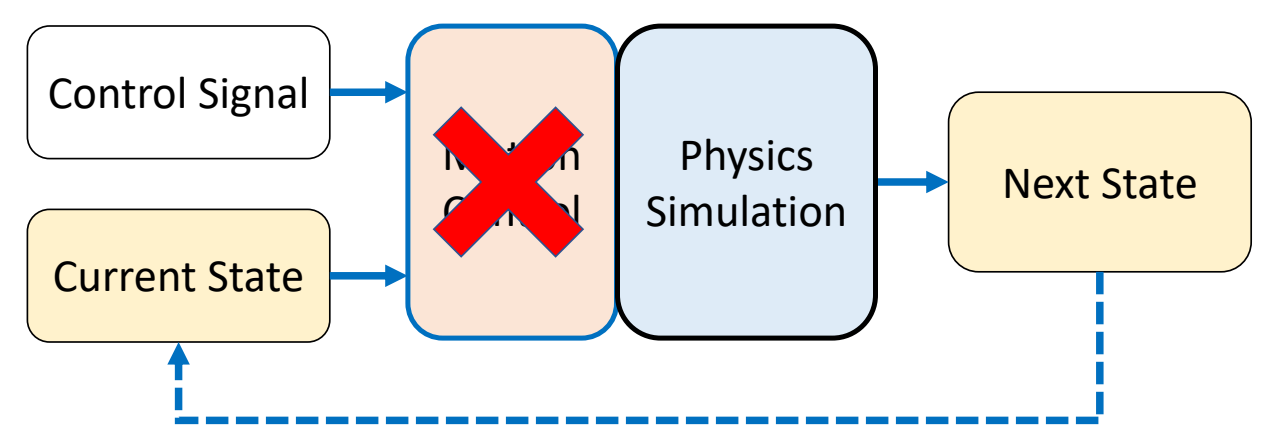
二、基于运动学的方法 (Kinematics-based Methods)
核心特征:直接从数据学习动作生成,不经过物理仿真,输出为关节姿态。
2.1 技术流派总览
运动学方法经过十余年发展,形成了四大主要流派:
flowchart TB
    subgraph Phase["流派一:相位系 (Phase-based)"]
        direction TB
        PFNN["PFNN (2017)"] --> LP["Local Phases (2020)"]
        LP --> SM["Style Modelling (2020)"]
        LP --> PM["Phase Manifolds (2023)"]
    end

    subgraph Trans["流派二:RTN (Transition Generation)"]
        direction TB
        RTN["RTN (2018)"]
    end

    subgraph MM["流派三:Motion Matching 系"]
        direction TB
        MM0["Motion Matching (2019)"] --> LMM["Learned MM (2020)"]
        LMM --> MOCHA["MOCHA (2023)"]
    end

    subgraph Diff["流派四:扩散模型系"]
        direction TB
        AMDM["A-MDM (2024)"] --> CAMDM["CAMDM (2024)"]
        CAMDM --> AAMDM["AAMDM (2024)"]
        AAMDM --> DART["DART (2025)"]
    end

    style Phase fill:#e1f5fe
    style Trans fill:#fff3e0
    style MM fill:#f0f0f0
    style Diff fill:#e8f5e9
关键洞察:Local Phases (2020) 是相位系的核心分支点 —— 一支朝风格转换方向发展(Style Modelling),另一支朝相位流形插值方向发展(Phase Manifolds)。
| 流派 | 核心思想 | 优势 | 局限 |
|---|---|---|---|
| 相位系 | 相位解耦动作状态 / 相位流形插值 | 流畅无 artifacts / 自然过渡 | 相位定义需领域知识 |
| RTN (Transition Generation) | RNN 连接两个状态 | 无需标注、固定内存 | 过渡长度固定 |
| Motion Matching 系 | 数据搜索/预测 | 工业验证质量高 | 内存/训练成本 |
| 扩散模型系 | 概率扩散生成 | 高质量多样性 | 推理速度挑战 |
2.2 流派一:相位系 (Phase-based Methods)
核心思想:引入相位变量 $\phi \in [0, 2\pi)$ 作为动作周期的隐式表示,用相位解耦不同动作状态或在相位空间进行插值。
演进路径:
flowchart LR
    subgraph Phase["相位表示分支"]
        PFNN --> FS["Few-shot Styles"]
        FS --> LP["Local Phases"]
        LP --> SM["Style Modelling"]
    end

    subgraph Manifold["相位流形分支"]
        LP --> PM["Phase Manifolds"]
    end
两大分支:
从演进路径可以看出,Local Phases (2020) 是核心分支点,衍生出两个方向:
| 分支 | 演进路径 | 核心目标 | 典型应用 |
|---|---|---|---|
| 相位表示分支 | PFNN → Local Phases → Style Modelling | 用相位解耦不同动作状态 | VR 化身、风格化动画 |
| 相位流形分支 | Local Phases → Phase Manifolds | 在相位空间进行插值 | 过渡生成、动作补间 |
统一框架:
| 演进阶段 | 代表论文 | 核心贡献 | 典型应用 |
|---|---|---|---|
| 全局相位 | PFNN (2017) | 相位函数化权重,避免 artifacts | 复杂地形 locomotion |
| 少样本风格 | Few-shot Styles (2018) | 残差适配器 + CP 分解 | 风格迁移 |
| 局部相位 | Local Phases (2020) | 每个身体部位独立相位 | 多接触交互 |
| 风格调制 | Style Modelling (2020) | 特征变换 + 局部相位 | 实时风格切换 |
| 相位流形 | Phase Manifolds (2023) | 相位流形插值与过渡生成 | 动作补间 |
两大分支:
从演进路径可以看出,Local Phases (2020) 是核心分支点,衍生出两个方向:
| 分支 | 演进路径 | 核心目标 | 典型应用 |
|---|---|---|---|
| 相位表示分支 | PFNN → Local Phases → Style Modelling | 用相位解耦不同动作状态 | VR 化身、风格化动画 |
| 相位流形分支 | Local Phases → Phase Manifolds | 在相位空间进行插值 | 过渡生成、动作补间 |
代表论文:
- PFNN (2017): 相位函数化权重
- Few-shot Locomotion Styles (2018): 残差适配器 + CP 分解,少样本风格学习
- Local Motion Phases (2020): 局部相位表示
- Style Modelling (2020): 特征变换 + 局部相位
- Phase Manifolds (2023): 相位流形插值
- RTN (2018): 循环转移网络,transition 生成
注意:MOCHA (2023) 虽然使用了 AdaIN 进行风格转换(继承自 Style Modelling),但其核心是 Neural Context Matcher 进行上下文匹配,不属于相位系,而是属于Motion Matching 系(见 2.4 节)。
注意:POMP (2023) 虽然使用相位表示,但其核心是物理一致运动生成,输出关节力矩并使用物理仿真器,属于动力学方法(见 3.8.3 节)。
2.2.1 PFNN: Phase-Functioned Neural Networks (SIGGRAPH 2017)
论文: 113.md
核心创新: 将相位从「网络输入特征」升级为「网络权重的参数化变量」
架构:
flowchart LR
    Input["输入:状态 + 控制 + 相位φ"] --> PhaseFunc["相位函数Θ(φ)"]
    PhaseFunc --> Weights["生成网络权重"]
    Weights --> Expert1["专家 1"]
    Weights --> Expert2["专家 2"]
    Weights --> Expert3["专家 3"]
    Expert1 & Expert2 & Expert3 --> Mix["混合输出"]
    Mix --> Output["输出:姿态/速度/触地"]
关键洞察:
- 相位作为权重参数,避免不同相位动作混合导致的 artifacts
- 使用 Cubic Catmull-Rom Spline 插值专家权重
- 地形数据增强:从平地 mocap 生成崎岖地形训练数据
优点:
- 相位解耦,避免 artifacts
- 仅 10MB 模型大小
- 实时 60 FPS
缺点:
- 仍需手工标注相位和步态标签
- 泛化能力有限,仅支持训练过的步态
2.2.2 Few-shot Locomotion Styles (EG 2018)
论文: 214.md
核心创新: 首个少样本风格学习框架,几秒视频即可学会新走路风格
背景: PFNN 需要大量数据训练每种新风格,但动画师通常只有几秒参考视频。
方法框架:
flowchart TB
    subgraph Stage1["第一阶段:预训练"]
        data1["8 种风格大量数据"]
        pfnn["PFNN 主干网络"]
        adapter["残差适配器"]
        agnostic["风格无关参数 β_ag"]
        specific["风格相关参数 β_s (8 套)"]
    end

    subgraph Stage2["第二阶段:少样本学习"]
        data2["新风格几秒视频"]
        freeze["冻结主干网络"]
        learn["只学习新残差适配器"]
        cp["CP 分解降维"]
    end

    data1 --> pfnn
    pfnn --> agnostic
    pfnn --> adapter
    adapter --> specific

    data2 --> learn
    freeze --> learn
    learn --> cp

    style Stage1 fill:#e1f5fe
    style Stage2 fill:#fff3e0
关键技术:
| 技术 | 作用 | 效果 |
|---|---|---|
| 残差适配器 | 分离风格无关/相关参数 | 只需学习少量新参数 |
| CP 分解 | 3D 张量分解为三个矩阵 | 参数从 4MB 降至 0.13MB (30 倍压缩) |
| 可变 Dropout | 根据数据量调整正则化 | 防止少样本过拟合 |
CP 分解公式:
$$ X_k = A D(k) B^T $$
- $A, B$: 与相位无关的矩形矩阵
- $D(k)$: 与相位相关的对角矩阵
训练数据:
- 预训练:8 种风格 × 23104 帧(愤怒、孩子气、沮丧、中性、老人、骄傲、性感、大摇大摆)
- 少样本:50 种新风格,每种仅 1-5 秒视频
性能:
- 推理时间:0.0011 秒/帧(约 900 FPS)
- 存储:每风格仅需 0.13MB
优点:
- 几秒视频即可学会新风格
- 支持实时生成
- 参数效率高,内存占用低
缺点:
- 仅支持 Homogeneous 迁移(走→走,不能走→跑)
- 无法处理非周期性动作
- 生成动作略平滑,丢失高频细节
与 PFNN 的继承关系:
- PFNN: 每风格单独训练,需要大量数据
- Few-shot: 添加残差适配器,风格无关参数共享
2.2.3 Local Motion Phases (SIGGRAPH 2020)
论文: 216.md
核心创新: 每个身体部位学习独立相位,支持多接触交互
背景: PFNN 的全局相位假设所有部位同步运动,无法处理多接触动作(如手扶墙、脚踩台阶)。
全局相位 vs 局部相位:
| 全局相位 | 局部相位 |
|---|---|
| 单一相位值 | 每个身体部位独立相位 |
| 适用于周期性 locomotion | 适用于多接触交互 |
| 相位手动标注 | 无监督学习相位 |
局部相位表示:
$$ \phi = {\phi_{left_foot}, \phi_{right_foot}, \phi_{left_hand}, \phi_{right_hand}, ...} $$
与 PFNN 的继承关系:
- PFNN: 全局相位,需手动标注
- Local Phases: 局部相位,无监督学习
- 共同点:相位作为解耦变量
优点:
- 支持多接触交互
- 相位自动学习
- 异步运动建模
缺点:
- 相位数量固定
- 新接触类型需要训练
2.2.4 Style Modelling: 特征变换与局部相位 (SIGGRAPH 2020)
论文: 211.md
核心创新: Feature-Wise Transformations + Local Motion Phases
架构:
flowchart LR
    motion["输入动作 x"] --> Enc["动作编码器"]
    style["风格代码 z"] --> StyleEnc["风格编码器"]
    Enc --> FWT["Feature-Wise Transformation"]
    StyleEnc --> FWT
    FWT --> Dec["动作解码器"]
    Dec --> out["风格化动作 y"]
AdaIN 公式:
$$ \text{AdaIN}(x, z) = \sigma(z) \cdot \frac{x - \mu(x)}{\sigma(x)} + \mu(z) $$
Local Motion Phases vs 全局相位:
| 全局相位 | 局部相位 |
|---|---|
| 单一相位值 | 每个身体部位独立相位 |
| 适用于周期性动作 | 适用于非同步动作 |
| 难以处理复杂动作 | 灵活处理多接触动作 |
与 PFNN 的继承关系:
- PFNN: 全局相位,适用于 locomotion
- Style Modelling: 局部相位,适用于更复杂动作
- 继承:相位作为解耦变量的思想
优点:
- 实时 60+ FPS
- 支持多种风格平滑过渡
- 少样本风格学习
缺点:
- 仅适用于 locomotion
- 极端风格可能失真
2.2.5 Phase Manifolds: 相位流形插值 (2023)
论文: 212.md
核心创新: 使用 Periodic Autoencoder 学习相位变量,在相位流形空间进行插值生成过渡动作
注意: 虽然本论文与 Style Modelling (211) 同样使用局部相位表示,但其核心是相位流形插值用于 transition 生成,与 POMP (112) 的物理一致运动生成不同,本论文属于运动学相位系。
架构:
flowchart TB
    start["起始帧 s"] --> PAE["Periodic<br/>Autoencoder"]
    target["目标帧 t"] --> PAE
    duration["过渡时长 T"] --> Interp["相位流形插值"]
    PAE --> PhaseS["起始相位φ_s"]
    PAE --> PhaseT["目标相位φ_t"]
    PhaseS --> Interp
    PhaseT --> Interp
    Interp --> MoE["Mixture of Experts"]
    MoE --> Motion["过渡动作序列"]
相位流形约束:
- 相位在单位圆上:$\phi \in [0, 2\pi)$
- 周期性:$\phi(t) = \phi(t + T)$
- 流形插值:$\phi_t = \text{slerp}(\phi_s, \phi_t, t)$(球面线性插值)
与 Style Modelling 的关系:
- 共同点: 都使用局部相位表示解耦身体部位
- 差异: Style Modelling 用于风格转换,Phase Manifolds 用于过渡生成
与 POMP 的差异:
- Phase Manifolds (212): 运动学过渡生成,输出关节位置
- POMP (112): 物理一致运动生成,输出关节力矩 + 物理仿真
优点:
- 生成自然流畅的过渡
- 支持用户约束(end effector 位置)
- 多样化过渡生成
缺点:
- 依赖训练数据
- 长过渡质量下降
- 无法处理物理交互
2.3 流派二:RTN: Recurrent Transition Networks (SIGGRAPH 2018)
论文: 210.md
核心创新: 首个专门为 transition 生成设计的未来感知(future-aware)深度循环网络
背景: 在大型游戏中,动画图(Animation Graph)需要大量 transition 动画。传统方法的问题:
- 手工制作 transition 非常耗时:动画师需要手动制作大量的过渡动画
- 内存占用大:Motion Graph 方法需要将动画数据和图结构加载到内存中
- 扩展性差:随着数据集增大,内存需求线性增长
- 需要标注:很多方法需要 gait、phase、contact 等标签
方法框架:
flowchart TB
    past["过去上下文<br/>10 帧"] --> Enc["Frame Encoder"]
    target["目标姿态<br/>归一化"] --> TargetEnc["Target Encoder"]
    offset["全局偏移<br/>目标 - 当前"] --> OffsetEnc["Offset Encoder"]

    Enc --> LSTM["改进的 LSTM<br/>512 单元"]
    TargetEnc --> LSTM
    OffsetEnc --> LSTM

    LSTM --> Dec["Frame Decoder"]
    Dec --> out["下一帧预测"]

    style Enc fill:#e1f5fe
    style LSTM fill:#fff3e0
    style Dec fill:#e8f5e9
核心架构:
| 组件 | 架构 | 作用 |
|---|---|---|
| Frame Encoder | 2 层 MLP, 512 单元 | 编码当前帧 + 地形(可选) |
| Target Encoder | 2 层 MLP, 128 单元 | 编码目标姿态(整序列恒定) |
| Offset Encoder | 2 层 MLP, 128 单元 | 编码目标与当前的差异 |
| Recurrent Generator | 改进 LSTM, 512 单元 | 添加未来上下文条件化权重 |
| Frame Decoder | 2 层 MLP | 输出下一帧 |
改进的 LSTM:
$$i_t = \alpha(W^{(i)}h^E_t + U^{(i)}h^R_{t-1} + C^{(i)}h^{F,O}t + b^{(i)})$$ $$o_t = \alpha(W^{(o)}h^E_t + U^{(o)}h^R{t-1} + C^{(o)}h^{F,O}t + b^{(o)})$$ $$f_t = \alpha(W^{(f)}h^E_t + U^{(f)}h^R{t-1} + C^{(f)}h^{F,O}_t + b^{(f)})$$ $$\hat{c}t = W^{(c)}h^E_t + W^{(c)}h^R{t-1} + C^{(c)}h^{F,O}t + b^{(c)}$$ $$c_t = f_t \odot c{t-1} + i_t \odot \tau(\hat{c}_t)$$ $$h^R_t = o_t \odot \tau(c_t)$$
关键设计:
- 添加了 $C^{(\cdot)}$ 权重用于未来上下文条件化
- Hidden State 初始化器:学习逆函数 $H(x_{past_first}) \to (h_0, c_0)$
- 地形感知:通过局部高度图(13×13 网格)实现崎岖地形导航
数据表示:
- 根节点相对位置:$\tilde{x}t = [v_t, j^t_1, ..., j^t{K-1}]^T$
- 根节点速度:$v_t = r_t - r_{t-1}$
- 标准化:$x_t = (\tilde{x}_t - \mu_x) / \sigma_x$
训练细节:
- Transition 长度:30 帧(1 秒)
- Past context:10 帧
- Future context:2 帧(目标姿态)
- 总窗口长度:50 帧
- 损失函数:$\mathcal{L} = \frac{1}{P} \sum_{t=1}^{P} ||x_{t+1} - \hat{x}_{t+1}||^2$
- 无需任何 gait、phase、contact 或 action 标签
优点:
- 自动生成高质量 transition,无需手工制作
- 固定大小的网络,内存占用恒定
- 无需任何标注即可训练
- 质量媲美 Mocap ground truth
缺点:
- Transition 长度固定,需要预设
- 自回归生成,推理速度取决于长度
- 无法处理复杂障碍物
与 PFNN 的对比:
- PFNN:相位条件化,生成连续 locomotion
- RTN:transition 专用,连接两个状态
- PFNN 需要相位标注,RTN 无需标注
应用场景:
- Animation Graph 的 transition 节点:替代手工制作的过渡动画
- 动画超分辨率:从 1fps 压缩动画恢复
- 地形导航:崎岖地形上的长 transition
2.4 流派三:Motion Matching 系
核心思想:从动作数据库搜索/预测最匹配当前状态的帧。
演进路径:
flowchart LR
    MM["Motion Matching (2019)<br/>工业标准"] --> LMM["Learned Motion Matching (2020)<br/>神经网络替代"]
    LMM --> MOCHA["MOCHA (2023)<br/>角色化扩展"]
Motion Matching 核心流程:
- 提取当前帧特征(姿势、速度、轨迹)
- 在数据库中搜索最近邻
- 返回对应帧并推进索引
Learned Motion Matching 创新:用三个神经网络替代数据库搜索,固定内存占用。
MOCHA 扩展:在 Learned Motion Matching 基础上,增加 Neural Context Matcher 实现角色风格转换和体型适配。
2.4.1 Learned Motion Matching (SIGGRAPH 2020)
论文: 208.md
核心创新: 用三个神经网络替代 Motion Matching 的数据库搜索
背景: Motion Matching 是游戏工业标准,但需要存储海量动画数据库,内存占用随数据量线性增长。
三网络功能:
| 网络 | 输入 | 输出 | 替代功能 |
|---|---|---|---|
| Decompressor | 特征向量 x + 潜变量 z | 姿态 y | Animation Database 查找 |
| Projector | 查询特征向量 | 最近邻索引 k* | 最近邻搜索 |
| Stepper | 当前索引 k* | 下一帧索引 | 数据库索引推进 |
优点:
- 保留 Motion Matching 的质量和可控性
- 固定内存占用(网络权重),不随数据量增长
- 已应用于多个 AAA 游戏
缺点:
- 训练时间比原始 Motion Matching 长
- 网络预测 vs 精确搜索有轻微质量损失
2.4.2 MOCHA: Real-Time Motion Characterization (SIGGRAPH Asia 2023)
论文: 209.md
核心创新: 首个实时角色表征框架,同时转换动作风格和身体比例
背景: 将中性动作转换为特定角色风格(如僵尸、公主、小丑),同时适配不同体型。
架构:
flowchart TB
    src["Source Motion<br/>中性动作"] --> BodyEnc["Bodypart Encoder<br/>6 身体部位"]
    BodyEnc --> SrcFeat["Source Feature"]
    SrcFeat --> NCM["Neural Context Matcher<br/>C-VAE + 自回归"]
    NCM --> CharFeat["Character Feature"]
    CharFeat --> Charz["Characterizer<br/>Transformer+AdaIN"]
    SrcFeat --> Charz
    Charz --> OutFeat["Translated Feature"]
    OutFeat --> Output["Characterized Motion"]
AdaIN 公式:
$$ \text{AdaIN}(z_{src}, z_{cha}) = \sigma(z_{cha}) \cdot \frac{z_{src} - \mu(z_{src})}{\sigma(z_{src})} + \mu(z_{cha}) $$
NCM Prior:
$$ p(s_i | z_{i-1}^{cha}, f(z_i^{src})) = \mathcal{N}(\mu, \sigma) $$
与 Style Modelling 的继承关系:
- Style Modelling: AdaIN 用于风格转换
- MOCHA: AdaIN + Transformer,同时处理风格 + 体型
优点:
- 实时 60 FPS
- 同时处理风格转换 + 身体比例适配
- 支持稀疏输入(VR tracker)
缺点:
- 训练数据中的角色有限,新角色需重新训练
- 极端风格可能失真
2.5 流派四:扩散模型系 (Diffusion-based Methods)
核心挑战:标准扩散模型需要 1000 步去噪,无法满足实时性要求(60 FPS)。
演进路径:
flowchart TB
    DM["标准扩散模型<br/>1000 步去噪"] --> AMDM["A-MDM (2024)<br/>自回归 +50 步"]
    DM --> CAMDM["CAMDM (2024)<br/>8 步 + 风格转换"]
    DM --> AAMDM["AAMDM (2024)<br/>5 步 DD-GAN+ADM"]
    AMDM --> DART["DART (2025)<br/>Latent Space Control"]

    subgraph 加速演进
    AMDM -.->|50 步 | CAMDM
    CAMDM -.->|8 步 | AAMDM
    AAMDM -.->|5 步 | DART
    end
加速策略对比:
| 方法 | 去噪步数 | 加速策略 | 实时性 |
|---|---|---|---|
| A-MDM | 50 步 | 自回归设计 | 30+ FPS |
| CAMDM | 8 步 | 条件化 + 引导采样 | 60+ FPS |
| AAMDM | 5 步 | DD-GAN+ADM 级联 | 60+ FPS |
| DART | ~20 步 | Latent 空间扩散 | 60+ FPS |
2.5.1 A-MDM: Auto-regressive Motion Diffusion Model (SIGGRAPH 2024)
论文: 206.md
核心创新: 将扩散模型从 space-time 重新设计为 auto-regressive
自回归公式:
$$ p(x_{1:T}) = \prod_{t=1}^{T} p(x_t | x_{1:t-1}) $$
架构: 简单 3 层 MLP,50 步去噪
控制套件:
- Task-oriented sampling
- Motion in-painting
- Keyframe in-betweening
- Hierarchical reinforcement learning
与 CAMDM 的差异:
- A-MDM: 强调控制套件,MLP 架构
- CAMDM: 强调风格转换,Transformer 架构
2.5.2 CAMDM: Conditional Autoregressive Motion Diffusion Model (SIGGRAPH 2024)
论文: 207.md
核心创新: 8 步去噪实现实时高质量多样角色动画
关键技术:
| 技术 | 作用 |
|---|---|
| 分离条件 Tokenization | 每个控制条件独立 token,避免特征主导 |
| Classifier-free guidance on history | 在历史动作上应用 guidance,实现风格转换 |
| 启发式轨迹扩展 | 回收上次预测轨迹,避免抖动 |
条件输入:
- 风格/步态
- 移动速度
- 朝向方向
- 未来轨迹
优点:
- 8 步去噪 ≈ 几毫秒,60+ FPS
- 支持多风格平滑转换
- 无需微调实现风格转换
缺点:
- 8 步去噪仍有优化空间
- 依赖 mocap 数据
2.5.3 AAMDM: Accelerated Auto-regressive Motion Diffusion Model (CVPR 2024)
论文: 204.md
核心创新: 5 步去噪 (3 DD-GAN + 2 ADM)
架构:
Autoencoder: 338D pose → 64D latent
      ↓
Generation Module: DD-GANs (3 步)
      ↓
Polishing Module: ADM (2 步)
      ↓
输出:高质量动作
总去噪步数: $T_{AA} = T_{GAN} + T_{ADM} = 3 + 2 = 5$
与 CAMDM 的差异:
- CAMDM: 8 步,强调风格转换
- AAMDM: 5 步,强调加速
2.5.4 DARTControl: Diffusion-based Autoregressive Motion Model (ICLR 2025)
论文: 205.md
核心创新: Motion Primitive 表示 + Latent Space Control
Motion Primitive:
- H=2 帧历史(与前一 primitive 重叠)
- F=8 帧未来
Latent Space Control 方法:
- 优化方法: latent noise optimization
- 学习方法: MDP + RL (PPO)
优势: 10x 加速 vs FlowMDM
与 A-MDM 的差异:
- A-MDM: 原始空间扩散
- DART: Latent 空间扩散,更高效
2.6 运动学方法总结
四大流派核心思想对比
| 流派 | 代表方法 | 核心贡献 | 典型应用 |
|---|---|---|---|
| 相位系 | PFNN → Few-shot Styles → Local Phases → Style Modelling → Phase Manifolds | 相位作为权重参数/条件输入,避免 artifacts | VR 化身、风格化动画、过渡生成 |
| RTN (Transition Generation) | RTN (2018) | RNN 连接两个状态 | 动画图 transition、超分辨率 |
| Motion Matching 系 | MM → Learned MM → MOCHA | 数据搜索/预测生成动作 + 角色化 | 游戏 NPC、在线游戏、角色设计 |
| 扩散模型系 | A-MDM → CAMDM → AAMDM → DART | 概率扩散模型生成 | 电影动画、多样性生成 |
流派选择指南
flowchart TD
    Q1["需要什么类型的控制?"] --> |风格转换 | A1["MOCHA / CAMDM / Style Modelling"]
    Q1 --> |稀疏输入 VR | A2["PFNN / MOCHA"]
    Q1 --> |高质量多样性 | A3["CAMDM / DART"]
    Q1 --> |低内存占用 | A4["Learned Motion Matching"]
    Q1 --> |transition 生成 | A5["RTN / Phase Manifolds"]
    Q1 --> |少样本学习 | A6["Few-shot Styles"]
运动学方法详细对比
| 方法 | 架构 | 去噪步数 | FPS | 风格转换 | 空间控制 | 物理感知 |
|---|---|---|---|---|---|---|
| PFNN | 混合专家 | N/A | 60+ | △ | △ | ✗ |
| Few-shot Styles (214) | 残差适配器+CP 分解 | N/A | 60+ | ✓ (少样本) | △ | ✗ |
| Local Motion Phases | 相位条件化 | N/A | 60+ | ✗ | △ | ✗ |
| Style Modelling | FWT+ 相位 | N/A | 60+ | ✓ | ✗ | ✗ |
| Phase Manifolds | MoE+PAE | N/A | 30+ | ✗ | ✓ | ✗ |
| RTN | LSTM | N/A | 60+ | ✗ | ✓ | △ |
| Learned MM | 三网络 | N/A | 60+ | ✗ | △ | ✗ |
| MOCHA | Transformer | N/A | 60+ | ✓ | ✗ | ✗ |
| A-MDM | MLP | 50 | 30+ | △ | △ | ✗ |
| CAMDM | Transformer | 8 | 60+ | ✓ | ✓ | ✗ |
| AAMDM | DD-GAN+ADM | 5 | 60+ | △ | ✗ | ✗ |
| DART | Latent Diffusion | ~20 | 60+ | ✓ | ✓ | ✗ |
2.7 常见问题解答 (FAQ)
Q1: 相位系的发展脉络是什么?
相位系是一个统一的方法论,其核心思想是引入相位变量 $\phi \in [0, 2\pi)$ 作为动作的解耦表示,通过相位来参数化网络权重或作为条件输入,避免不同动作状态的混合导致 artifacts。
统一演进框架:
| 阶段 | 代表论文 | 核心创新 | 相位角色 |
|---|---|---|---|
| 全局相位 | PFNN (2017) | 相位函数化网络权重 | 权重参数化变量 |
| 少样本风格 | Few-shot Styles (2018) | 残差适配器 + CP 分解 | 风格条件 |
| 局部相位 | Local Phases (2020) | 每个身体部位独立相位 | 多接触解耦 |
| 风格调制 | Style Modelling (2020) | 特征变换 + 局部相位 | 风格注入条件 |
| 相位流形 | Phase Manifolds (2023) | 周期自编码学习相位流形 | 流形空间坐标 |
关键洞察:
- Local Phases (2020) 是核心分支点,同时影响了 Style Modelling(风格转换)和 Phase Manifolds(过渡生成)两个方向
- 相位系内部的区别仅在于相位的使用方式(全局 vs 局部、解耦 vs 流形插值),但核心思想统一
注意:POMP (2023) 虽然使用相位表示,但其核心是物理一致运动生成,输出关节力矩并使用物理仿真器,属于动力学方法(见 3.8.3 节)。
Q2: MOCHA 属于哪个流派?
MOCHA 属于 Motion Matching 系,而不是相位系。理由如下:
| 维度 | 相位系 | MOCHA |
|---|---|---|
| 核心机制 | 相位作为权重参数或输入特征 | Neural Context Matcher 上下文匹配 |
| 相位使用 | 显式相位变量 $\phi$ | 无显式相位,用上下文特征条件化 |
| 继承关系 | PFNN → Local Phases → Style Modelling | Motion Matching → Learned MM → MOCHA |
MOCHA 的核心贡献:
- Neural Context Matcher: 用 C-VAE + 自回归生成替代数据库搜索
- Characterizer: 用 AdaIN + Cross-Attention 实现风格转换和体型适配
注意:MOCHA 虽然使用了 AdaIN(继承自 Style Modelling),但这只是风格注入的工具,其核心架构是基于上下文匹配的,因此属于 Motion Matching 系。
Q3: RTN 属于什么系?
RTN 不属于任何主要流派,它是一个专用场景方法:
| 维度 | RTN | 三大流派 |
|---|---|---|
| 目标场景 | Transition 生成 | 连续 locomotion |
| 相位需求 | 无需相位 | 需要相位或类似机制 |
| 标注需求 | 无需任何标注 | 通常需要相位/步态标注 |
| 网络结构 | 改进 LSTM | 多样化(混合专家、Transformer、扩散) |
RTN 的定位:
- RTN 是一个特殊的存在,专门处理游戏动画图中的transition 生成问题
- 它不属于相位系(无需相位)、不属于 Motion Matching 系(不用搜索)、不属于扩散模型系(2018 年工作)
- 在流派选择指南中,RTN 作为"transition 生成"的专用方案被推荐
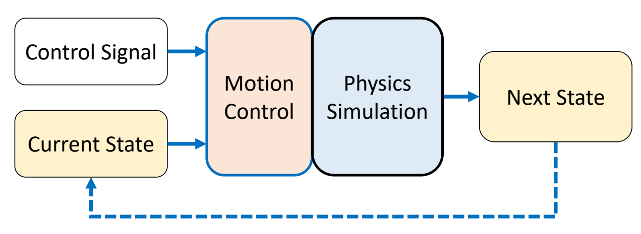
三、基于动力学的方法 (Dynamics-based Methods)
核心特征: 输出为关节力矩或 PD 控制目标,需要物理仿真器执行。
3.1 技术演进时间线
timeline
    title 动力学方法发展时间线
    2010 : Feature-Based : 高层物理特征
    2017 : DeepLoco : 分层 RL+ 环境感知
    2018 : DeepMimic : RL+ 模仿
    2018 : Mode-Adaptive : 四足统一控制
    2019 : DReCon : MM+RL
    2021 : AMP : 对抗运动先验
    2022 : ASE : 预训练技能库
    2023 : ControlVAE : 状态条件先验
    2023 : Perpetual : 实时虚拟化身
    2023 : UniRep : 统一表示 + 蒸馏
    2024 : PDP/DiffuseLoco : 扩散策略
    2024 : MaskedMimic : 掩码运动补全
    2025 : PARC : 迭代数据扩增
    2025 : UniPhys : 统一规划 + 控制
3.2 核心思想继承关系
动力学方法经过十余年发展,形成了四条主要演进主线:
flowchart TB
    subgraph RL["RL lineage"]
        FB["Feature-Based"] --> DL["DeepLoco"]
        DL --> DM["DeepMimic"]
        DM --> AMP["AMP"]
        AMP --> ASE["ASE"]
    end

    subgraph Hybrid["Hybrid lineage"]
        DL --> DReCon["DReCon<br/>MM+RL"]
        DM --> DReCon
        DReCon --> PDP["PDP<br/>RL 专家蒸馏"]
    end

    subgraph Pretrain["Pretraining lineage"]
        ASE --> CVAE["ControlVAE"]
        ASE --> UniRep["Universal Representation"]
    end

    subgraph Diffusion["Diffusion lineage"]
        PDP --> DiffuseLoco["DiffuseLoco"]
        ASE --> MaskedMimic["MaskedMimic"]
        MaskedMimic --> UniPhys["UniPhys"]
        DReCon --> PARC["PARC<br/>迭代扩增"]
    end
四条演进主线详解
| 主线 | 演进路径 | 核心问题 | 解决方案 |
|---|---|---|---|
| RL Lineage | DeepLoco → DeepMimic → AMP → ASE | 如何从数据学习控制策略? | 分层 RL → RL 模仿 → 对抗学习 → 预训练技能库 |
| Hybrid Lineage | DeepLoco → DReCon → PDP | 如何统一多技能控制? | 分层架构 → 动态参考选择 → 多专家蒸馏 |
| Pretraining Lineage | ASE → ControlVAE → UniRep | 如何提高样本效率? | 对抗预训练 → 状态条件先验 → Prior+ 蒸馏 +RL 范式 |
| Diffusion Lineage | PDP → DiffuseLoco / ASE → MaskedMimic → UniPhys / DReCon → PARC | 2024 年扩散模型如何应用? | 扩散策略 / 掩码补全 / 迭代扩增 |
关键洞察:
- DeepLoco (2017) 是分层 RL 的开创者,首次实现环境感知(32×32 高度图)+ 双控制器架构(HLC 规划 + LLC 执行)
- DeepMimic (2018) 是深度学习时代的起点,首次证明 RL+ 模仿可以学习高质量动态动作(后空翻、旋转)
- AMP (2021) 解决数据标注问题,从需要精确跟踪 → 无标注对抗学习
- ASE (2022) 解决技能复用问题,预训练的技能库可以微调至下游任务
- DReCon (2019) 开创混合控制范式,生成器 (MM) + 跟踪器 (RL) 的架构被 PDP/PARC 继承
- 2024 年趋势:扩散模型成为主流(DiffuseLoco、MaskedMimic、UniPhys、PARC)
3.3 主线一:RL 模仿学习 (RL Lineage)
演进路径: Feature-Based Control (2010) → DeepLoco (2017) → DeepMimic (2018) → AMP (2021) → ASE (2022)
3.3.1 Feature-Based Control (SIGGRAPH 2010)
论文: 200.md
核心思想: 用高层物理特征设计控制器
方法框架:
flowchart LR
    Define["定义特征"] --> Obj["设计目标函数"]
    Obj --> Priority["优先级优化"]
    Priority --> Solve["求解关节力矩τ"]
关键公式:
- Setpoint 目标:$E(x) = ||\ddot{y}_d - \ddot{y}||^2$
- 角动量目标:$E_{AM}(x) = ||\dot{L}_d - \dot{L}||^2$
- 优先级优化:$h_i = \min_x E_i(x)$ s.t. $E_k(x) = h_k, \forall k < i$
优点: 可解释、无需数据 缺点: 实现复杂、动态性差
3.3.2 DeepLoco (SIGGRAPH 2017)
论文: 218.md
核心创新: 分层深度强化学习 + 环境感知
方法框架:
flowchart TB
    Terrain["32×32 地形图"] --> HLC["高层控制器 HLC<br/>2Hz 规划步法"]
    HLC -->|"p̂₀, p̂₁, θ̂_root"| LLC["低层控制器 LLC<br/>30Hz 执行动作"]
    LLC --> PD["PD 控制器"]
    PD --> Sim["物理仿真"]
分层架构:
| 控制器 | 频率 | 输入 | 输出 |
|---|---|---|---|
| HLC | 2Hz | 地形图 + 任务目标 | 步法计划 (p̂₀, p̂₁, θ̂_root) |
| LLC | 30Hz | 状态 + 步法计划 | 关节 PD 目标 |
关键技术:
- 双线性相位变换: 将相位φ分 4 区间,强制不同阶段用不同子网络
- 参考动作引导: 不精确跟踪,只模仿风格
- 迁移学习: 同一 LLC 可复用多个 HLC 任务
优点: 环境感知、多任务支持、组件可复用 缺点: 训练时间长 (LLC 2 天+HLC 7 天)、采样效率低
3.3.3 DeepMimic (SIGGRAPH 2018)
论文: 201.md
核心创新: 深度 RL + 模仿学习
方法框架:
flowchart LR
    Mocap["参考动作 mocap"] --> Reward["定义奖励 r^I+r^G"]
    Reward --> PPO["PPO 训练π(a|s)"]
    PPO --> PD["PD 控制器执行"]
    PD --> Sim["物理仿真"]
模仿奖励:
$$ r^I_t = w_p r^p_t + w_v r^v_t + w_e r^e_t + w_c r^c_t $$
训练技巧:
- RSI (Reference State Initialization): 从参考动作随机状态开始
- ET (Early Termination): 跌倒立即终止
- 相位条件化: $\phi_t = (t \mod T_{cycle}) / T_{cycle}$
优点: 动作质量高、可学习动态动作 缺点: 每技能单独训练、样本效率低
3.4 主线二:混合控制 (Hybrid Lineage)
演进路径: DReCon (2019) → PDP (2024) → PARC (2025)
核心思想: 生成器(选择/生成参考轨迹)+ RL 跟踪器(保证物理稳定性)。
3.4.1 DReCon (SIGGRAPH Asia 2019)
论文: 190.md
核心架构:
flowchart LR
    MM["Motion Matching"] --> RL["RL 规划"]
    RL --> PD["PD 执行"]
    PD --> Sim["物理仿真"]
    Sim --> MM
创新点:
- 用 Motion Matching 替代 mocap 参考轨迹
- RL 输出 PD 目标而非直接力矩
- 支持实时响应
与 DeepMimic 的差异:
- DeepMimic: 跟踪单一 mocap 片段
- DReCon: 用 Motion Matching 选择参考轨迹
3.3.3 AMP: Adversarial Motion Priors (SIGGRAPH 2021)
论文: 198.md
核心创新: 用对抗学习从无标注数据学习
方法框架:
flowchart LR
    Data["无标注 mocap"] --> D["判别器 D(s,s')"]
    D --> Policy["策略π"]
    Policy --> Adv["对抗奖励-log(1-D)"]
    Adv --> Policy
对抗奖励:
$$ r_{adv} = -\log(1 - D(s_t, s_{t+1})) $$
AMP 的核心优势:
- 无需精确跟踪参考动作
- 能够从多样化数据集学习
- 自动学习技能组合
局限性:
- 训练不稳定(对抗博弈)
- GAN+RL 训练难度大
3.3.4 ASE: Adversarial Skill Embeddings (SIGGRAPH 2022)
论文: 199.md
核心创新: 预训练通用技能库 + 下游微调
两阶段训练:
flowchart TB
    subgraph PreTrain["阶段 1: 预训练"]
        Data["无标注数据集"] --> LowPolicy["低级策略π(a|s,z)"]
        Data --> Discriminator["对抗 + 互信息"]
    end

    subgraph TaskTrain["阶段 2: 任务训练"]
        Goal["任务目标 g"] --> HighPolicy["高级策略ω(z|s,g)"]
        LowPolicyFixed["低级策略 (固定)"] --> Output["输出动作 a"]
        HighPolicy --> LowPolicyFixed
    end

    PreTrain --> TaskTrain
预训练目标:
$$ \max_{\pi} -D_{JS}(d_{\pi} || d_M) + \beta I(s, s'; z | \pi) $$
与 AMP 的差异:
- AMP: 每任务从头训练
- ASE: 预训练可复用,技能库学习
优点: 技能可复用、支持插值和组合 缺点: 需要大规模并行模拟(Isaac Gym)
3.5 特殊应用:四足动物控制 (Mode-Adaptive)
论文: 213.md
核心创新: 单个神经网络处理多种四足动物步态
架构:
flowchart TB
    state["角色状态"] --> ModeEst["Mode 估计"]
    cmd["用户命令"] --> ModeEst
    terrain["地形信息"] --> ModeEst
    ModeEst --> Adaptive["Adaptive 权重"]
    state --> Control["控制器"]
    cmd --> Control
    Adaptive --> Control
    Control --> Action["关节目标"]
优点:
- 流畅的步态切换
- 适应不同地形
- 自然运动质量
缺点:
- 仅适用于四足动物
- 需要 mocap 数据
3.6 主线三:预训练与统一表示 (Pretraining Lineage)
演进路径: ControlVAE (2023) → UniRep (2023) → MaskedMimic (2024) → UniPhys (2025)
3.6.1 ControlVAE (TOG 2023)
论文: 202.md
核心创新: 状态条件先验 + 世界模型
与 ASE 对比: | 维度 | ASE | ControlVAE | |------|-----|------------| | 先验类型 | 球面均匀分布 | 状态条件高斯 | | 学习方式 | 对抗 + 互信息 | 世界模型 + ELBO | | 技能表示 | 离散技能库 | 连续潜在空间 |
3.6.2 UniRep: Universal Humanoid Motion Representations (2023)
论文: 191.md
核心创新: 建立 Prior + Distillation + RL 的标准范式,用 CVAE 学习动作先验,再蒸馏进物理稳定的 Decoder
三阶段训练:
flowchart TB
    Mocap["MoCap 数据"] --> CVAE["CVAE 训练"]
    CVAE --> Prior["动作先验 z"]

    TO["轨迹优化器"] --> Stable["物理稳定轨迹"]
    Stable --> Distill["蒸馏到 Decoder"]

    Prior --> RL["高层 RL"]
    Distill --> RL
核心困境解决:
- MoCap 生成模型:动作自然但物理不稳定
- 纯轨迹优化:物理稳定但动作单调
方案: 用蒸馏将物理稳定性灌进网络,保留 z 的多样性
优点:
- 定型并普及了 Prior + Distillation + RL 的标准流水线
- 动作自然性与物理稳定性兼顾
缺点:
- 能力上限受限于轨迹优化器的求解能力
- 仅覆盖简单 Locomotion(走、跑、转向等)
3.7 特殊应用:实时虚拟化身 (Perpetual)
论文: 196.md
核心创新: 实时虚拟化身控制系统
系统架构:
flowchart LR
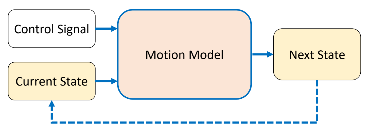
Input["视频/动捕/控制信号"] --> MotionGen["运动生成"]
MotionGen --> Track["物理跟踪控制器"]
Track --> Output["物理稳定全身控制"]
Output --> Disturb["扰动恢复"]
Disturb --> Track
特点:
- Meta 出品,面向 VR/AR 应用
- 实时优先,支持多种输入源
- 物理感知保证可行性
定位: 实时系统应用,不属于上述演进主线
3.8 主线四:扩散策略 (Diffusion Lineage)
演进路径: DiffuseLoco (2024)
核心思想: 使用扩散模型学习物理一致的控制策略。
3.8.1 DiffuseLoco (2024)
论文: 195.md
方法框架:
flowchart LR
    Data["离线 mocap"] --> Diff["扩散模型π(a|s,goal)"]
    Diff --> Distill["蒸馏 RL 策略"]
    Distill --> Control["实时控制"]
优点: 离线训练、无需在线 RL
3.8.2 POMP: Physics-consistent Motion Prior (CVPR 2024)
论文: 112.md
核心创新: 基于相流形的物理一致运动先验,将动力学模块置于训练循环外
注意: POMP 虽然使用相位表示(类似相位系),但其核心是物理一致的运动生成,输出关节力矩并使用物理仿真器,因此属于动力学方法而非运动学相位系。
架构:
flowchart TB
    subgraph Input["输入"]
        state["角色状态 + 地形 + 轨迹"]
    end

    subgraph Kinematic["运动学模块"]
        MoE["OrthoMoE Encoder"]
        Diff["Diffusion Decoder"]
    end

    subgraph Dynamic["动力学模块"]
        IK["逆动力学 PD 控制"]
        FK["前向动力仿真"]
    end

    subgraph Phase["相位编码模块"]
        PAE["Periodic Autoencoder"]
        Align["语义对齐"]
    end

    Input --> MoE
    MoE --> Diff
    Diff --> IK
    IK --> FK
    FK --> Align
    Align --> PAE
    PAE --> MoE

    style Kinematic fill:#e1f5fe
    style Dynamic fill:#fff3e0
    style Phase fill:#e8f5e9
三模块协作:
- 运动学模块: 基于扩散的运动先验生成初始姿态
- 动力学模块: 物理仿真确保物理合理性(接触力、碰撞)
- 相位编码模块: 将仿真姿态投影回运动先验的相流形
关键洞察:
- 直接反馈仿真结果会导致误差累积
- 相流形中的语义对齐解决领域鸿沟问题
- 动力学模块在训练循环外,计算高效
优点:
- 物理一致的运动生成
- 实时响应物理扰动
- 计算高效(动力学模块在训练循环外)
缺点:
- 依赖地形和冲量数据提取
- 复杂交互质量受限
3.8.3 PDP: Physics-Based Character Animation via Diffusion Policy (2024)
论文: 192.md
核心: RL 专家蒸馏 + 扩散策略
两阶段训练:
- 训练多个单任务 RL 专家
- 离线行为克隆蒸馏到单一 Diffusion Policy
与 DReCon 的继承关系:
- DReCon: Motion Matching + RL
- PDP: RL 专家 + Diffusion Policy
3.8.4 MaskedMimic (SIGGRAPH Asia 2024)
论文: 183.md
核心创新: 掩码运动补全统一多模态控制
CVAE 架构:
- 输入:多模态控制信号(掩码关键帧、对象、文本等)
- 输出:物理一致的 PD 控制目标
特点:
- 无需奖励工程
- 支持无缝任务切换
- 实时响应能力
与 UniPhys 的对比:
- MaskedMimic: 掩码补全范式
- UniPhys: Diffusion Forcing 范式
3.8.5 PARC (SIGGRAPH 2025)
论文: 189.md
核心创新: 基于物理仿真的迭代数据扩增框架
迭代循环:
flowchart TB
    Gen["Motion Generator<br/>扩散模型"] --> Synth["合成新地形轨迹"]
    Synth --> Track["Motion Tracker<br/>RL 物理修正"]
    Track --> Filter["质量筛选"]
    Filter --> Dataset["数据集扩增"]
    Dataset --> Gen
四项关键机制防止性能退化:
- 固定采样比例: 保留原始 mocap 作为监督锚点
- 物理约束修正: RL 控制器修正为物理可信运动
- 质量筛选: 仅保留成功样本
- 小步迭代: 微调策略,防止分布漂移
应用场景: 敏捷地形穿越(如跑酷)
与 DReCon 的继承关系:
- DReCon: Motion Matching + RL 跟踪
- PARC: 扩散生成 + RL 跟踪 + 迭代扩增
3.8.6 UniPhys (2025)
论文: UniPhys: Unified Planner and Controller with Diffusion (2025)
核心创新: 统一规划器 + 控制器,Diffusion Forcing 范式
方法框架:
flowchart LR
    Mocap["mocap 数据"] --> Preprocess["PD 控制预处理"]
    Preprocess --> GT["物理合理 GT<br/>动作略僵硬"]
    GT --> Train["训练 Diffusion 模型"]
    MultiModal["多模态输入<br/>文本/轨迹/目标"] --> Infer["引导采样推理"]
    Train --> Infer
    Infer --> Output["物理合理运动"]
与 MaskedMimic 对比: | 维度 | MaskedMimic | UniPhys | |------|-------------|---------| | 训练范式 | 掩码补全 | Diffusion Forcing | | PD 目标来源 | mocap+ 跟踪 | mocap+PD 预处理 | | 长序列处理 | 较短序列 | 噪声历史去噪 |
优点:
- 无需强化学习和蒸馏
- 训练简单,单模型推理
- 物理合理但动作略僵硬
3.9 动力学方法对比
| 方法 | 训练范式 | 样本效率 | 动作质量 | 抗扰动 | 实时性 |
|---|---|---|---|---|---|
| Feature-Based | 无需训练 | N/A | 中 | 中 | ✓ |
| DeepLoco | 分层 RL | 低 | 高 | 高 | ✓ |
| DeepMimic | RL+ 模仿 | 低 | 极高 | 高 | ✓ |
| Mode-Adaptive | 模仿学习 | 中 | 高 | 高 | ✓ |
| DReCon | RL+MM | 中 | 高 | 高 | ✓ |
| AMP | 对抗学习 | 低 | 极高 | 高 | ✓ |
| ASE | 预训练 + 微调 | 高 | 极高 | 高 | ✓ |
| ControlVAE | 世界模型 | 高 | 高 | 高 | ✓ |
| Perpetual | 实时跟踪 | 高 | 高 | 高 | ✓ |
| UniRep | Prior+ 蒸馏 +RL | 高 | 高 | 高 | ✓ |
| DiffuseLoco | 离线蒸馏 | 高 | 极高 | 高 | ✓ |
| PDP | RL 专家蒸馏 | 中 | 极高 | 高 | ✓ |
| MaskedMimic | 掩码补全 | 高 | 极高 | 高 | ✓ |
| PARC | 迭代扩增 | 高 | 极高 | 高 | ⚠️ |
| UniPhys | 直接训练 | 高 | 高 | 高 | ⚠️ |
四、运动学 vs 动力学:技术选型指南
4.1 核心差异
| 维度 | 运动学方法 | 动力学方法 |
|---|---|---|
| 输出 | 关节姿态/速度 | 关节力矩/PD 控制目标 |
| 物理仿真 | 否 | 是 |
| 真实感来源 | 数据驱动 | 物理约束 + 数据 |
| 抗扰动能力 | 无 | 强 |
| 环境交互 | 有限 | 强 |
| 训练成本 | 低 - 中 | 中 - 高 |
| 实现难度 | 低 | 高 |
4.2 思想演进总结
运动学方法演进主线
-
相位表示线 (PFNN → Style Modelling → MOCHA → Phase Manifolds)
- 核心思想:用相位解耦不同动作状态
- 演进:全局相位 → 局部相位 → 相位流形插值
-
Motion Matching 线 (MM → Learned MM → MOCHA)
- 核心思想:用数据搜索生成动作
- 演进:数据库搜索 → 神经网络预测 → 角色化扩展
-
扩散模型线 (A-MDM → CAMDM → AAMDM → DART)
- 核心思想:扩散模型高质量生成
- 演进:1000 步 → 50 步 → 8 步 → 5 步,同时支持实时控制
动力学方法演进主线
-
RL 模仿线 (DeepMimic → AMP → ASE)
- 核心思想:从 mocap 数据学习控制策略
- 演进:单技能跟踪 → 对抗先验 → 预训练技能库
-
混合控制线 (DReCon → PDP → PARC)
- 核心思想:生成器 + RL 跟踪
- 演进:Motion Matching → RL 专家 → 扩散模型 + 迭代扩增
-
统一表示线 (ControlVAE → UniRep → MaskedMimic → UniPhys)
- 核心思想:统一潜在空间表示
- 演进:状态条件先验 → Prior+ 蒸馏 → 掩码补全 → Diffusion Forcing
4.3 应用场景推荐
| 应用场景 | 推荐方法 | 理由 |
|---|---|---|
| 游戏 NPC | DeepMimic / ASE / Learned MM | 实时、质量高、抗扰动 |
| 电影动画 | CAMDM / DART / MOCHA | 多样性、风格控制、无需物理 |
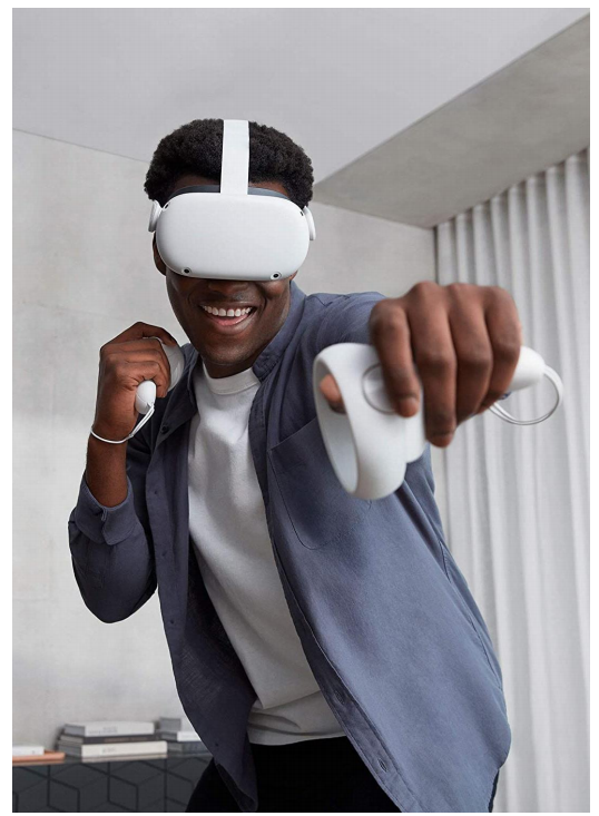
| VR 化身 | PFNN / CAMDM / MOCHA / Perpetual | 低延迟、稀疏输入支持 |
| 机器人仿真 | Feature-Based + RL / ASE | 安全、可解释、物理正确 |
| 在线游戏 | Learned Motion Matching | 低内存、服务器友好 |
| 角色设计 | MOCHA / Style Modelling | 风格转换、体型适配 |
| 四足动物 | Mode-Adaptive | 统一多步态控制 |
| 敏捷地形 | PARC / RTN (地形版) | 复杂地形穿越 |
| 多任务控制 | MaskedMimic / UniPhys | 统一框架处理多模态输入 |
4.4 方法选择决策树
flowchart TD
    Q1["需要物理仿真/抗扰动?"] --> |否 | A1["运动学方法"]
    Q1 --> |是 | A2["动力学方法"]

    A1 --> Q2["需要风格转换?"]
    Q2 --> |是 | A3["MOCHA / Style Modelling / CAMDM"]
    Q2 --> |否 | A4["PFNN / Learned MM / AAMDM"]

    A2 --> Q3["有无标注数据?"]
    Q3 --> |无 | A5["AMP / ASE"]
    Q3 --> |有 | A6["DeepMimic / DiffuseLoco"]

    A6 --> Q4["需要多模态控制?"]
    Q4 --> |是 | A7["MaskedMimic / UniPhys"]
    Q4 --> |否 | A8["PDP / DiffuseLoco"]

    A2 --> Q5["需要敏捷地形穿越?"]
    Q5 --> |是 | A9["PARC"]
五、开放性问题与未来趋势
5.1 技术挑战
-
实时性与质量权衡
- 扩散模型推理速度仍是瓶颈
- 方向:一致性模型、蒸馏、更少去噪步数
-
长时序规划
- 当前方法多为短时域反应式
- 方向:分层控制、世界模型、Diffusion Forcing
-
多角色泛化
- 技能绑定特定形态
- 方向:形态无关表示、零样本迁移
-
与语言模型结合
- 自然语言指令驱动
- 方向:LLM + 运动生成联合训练
-
在线适应
- 适应新环境、新扰动
- 方向:Test-Time Training、元学习、迭代扩增(如 PARC)
5.2 未来趋势
-
运动学 + 动力学融合
- 运动学方法生成参考轨迹
- 动力学方法保证物理可行性
- 代表工作:UniPhys、PARC
-
世界模型 + 扩散
- 学习可微物理引擎
- 在 latent space 规划
-
多模态大模型
- 视觉 + 语言 + 运动联合训练
- 具身智能 (Embodied AI)
-
自动技能发现
- 无监督发现技能层级
- 类似 LLM 的 emergent abilities
-
数据高效学习
- 少样本风格学习
- 迭代数据扩增(PARC 范式)
六、关键论文索引
运动学方法
| 论文 | 年份 | 链接 | 核心贡献 |
|---|---|---|---|
| PFNN | 2017 | 113 | 相位函数化权重 |
| Few-shot Locomotion Styles | 2018 | 214 | 残差适配器 +CP 分解,少样本风格学习 |
| Local Motion Phases | 2020 | 216 | 局部相位表示 |
| RTN | 2018 | 210 | 循环转移网络 |
| Style Modelling | 2020 | 211 | 特征变换 + 局部相位 |
| Learned Motion Matching | 2020 | 208 | 神经网络替代数据库 |
| MOCHA | 2023 | 209 | 上下文匹配角色化 |
| Phase Manifolds | 2023 | 212 | 相位流形中间帧 |
| POMP | 2023 | 112 | 物理一致运动先验 |
| A-MDM | 2024 | 206 | 自回归扩散模型 |
| CAMDM | 2024 | 207 | 8 步去噪 + 风格转换 |
| AAMDM | 2024 | 204 | 5 步 DD-GAN+ADM |
| DARTControl | 2025 | 205 | 潜在空间控制 |
动力学方法
| 论文 | 年份 | 链接 | 核心贡献 |
|---|---|---|---|
| Feature-Based Control | 2010 | 200 | 高层物理特征控制 |
| DeepMimic | 2018 | 201 | RL+ 模仿学习 |
| Mode-Adaptive | 2018 | 213 | 四足动物统一控制 |
| DReCon | 2019 | 190 | Motion Matching+RL |
| AMP | 2021 | 198 | 对抗运动先验 |
| ASE | 2022 | 199 | 预训练技能嵌入 |
| ControlVAE | 2023 | 202 | 状态条件先验 |
| Perpetual | 2023 | 196 | 实时虚拟化身 |
| UniRep | 2023 | 191 | 统一表示 + 蒸馏 |
| DiffuseLoco | 2024 | 195 | 扩散策略 |
| PDP | 2024 | 192 | RL 专家蒸馏 |
| MaskedMimic | 2024 | 183 | 掩码运动补全 |
| PARC | 2025 | 189 | 迭代数据扩增 |
| UniPhys | 2025 | 184 | 统一规划 + 控制 |
七、总结
角色位移控制领域呈现双轨并行、多线演进的发展态势:
运动学方法沿四大主线演进:
- 相位系:PFNN 的相位函数化权重 (2017) → Few-shot Styles 的残差适配器 +CP 分解 (2018) → Local Motion Phases 的局部相位 (2020) → Style Modelling 的特征变换 (2020) → Phase Manifolds 的相位流形插值 (2023)
- RTN (Transition Generation): 循环转移网络 (2018),专用 transition 生成
- Motion Matching 系:工业界标准 Motion Matching → Learned Motion Matching 的神经网络替代 → MOCHA 的上下文匹配角色化
- 扩散模型系:A-MDM 的自回归设计 → CAMDM 的 8 步去噪 + 风格转换 → AAMDM 的 5 步加速 → DART 的潜在空间控制
动力学方法沿三条主线演进:
- RL 模仿线:DeepMimic 的 RL+ 模仿 → AMP 的对抗先验 → ASE 的预训练技能库
- 混合控制线:DReCon 的 Motion Matching+RL → PDP 的 RL 专家蒸馏 → PARC 的扩散生成 + 迭代扩增
- 统一表示线:ControlVAE 的状态条件先验 → UniRep 的 Prior+ 蒸馏范式 → MaskedMimic 的掩码补全 → UniPhys 的 Diffusion Forcing
融合趋势:2024-2025 年的工作开始探索运动学 + 动力学的融合:
- UniPhys 用 PD 预处理保证物理合理性
- PARC 用迭代扩增结合生成与物理修正
- Perpetual 实现实时物理跟踪
这将是未来的重要方向。
参考文献: 详见各论文笔记文件
本文出自CaterpillarStudyGroup,转载请注明出处。
P2
Outline
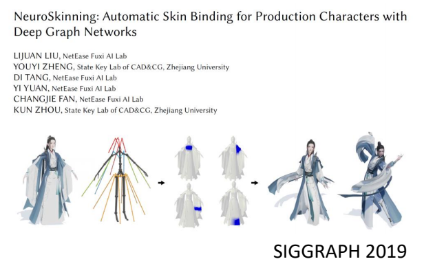
🔎 SIGGRAPH 经典的蒙皮课程。
Many images are from: https://skinning.org/
Alec Jacobson, Zhigang Deng, Ladislav Kavan, and J. P. Lewis. 2014.
Skinning: real-time shape deformation.
In ACM SIGGRAPH 2014 Courses (SIGGRAPH '14)
P7
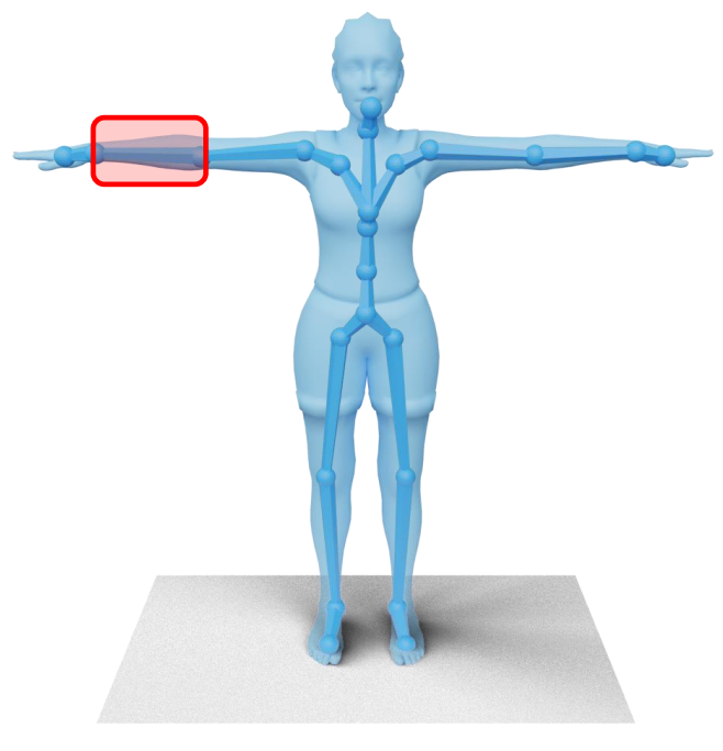
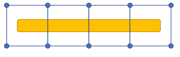
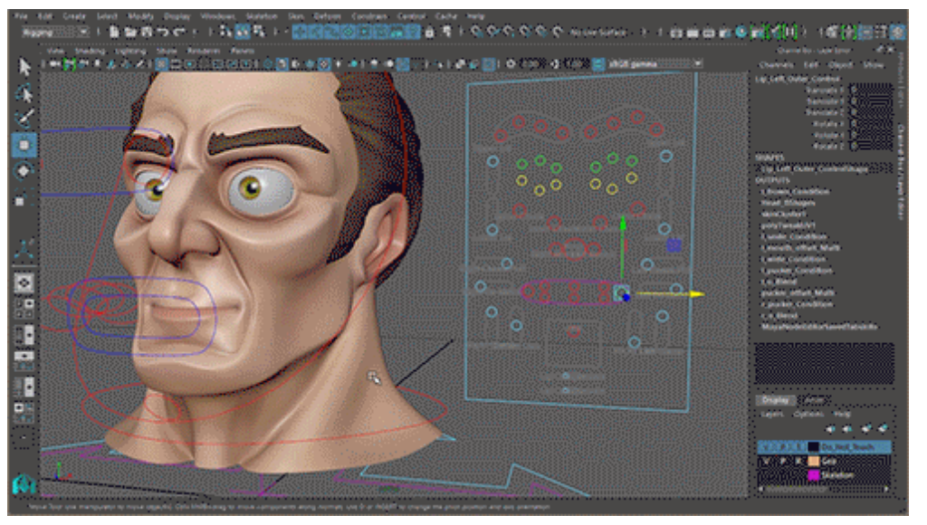
Skinning Deformation
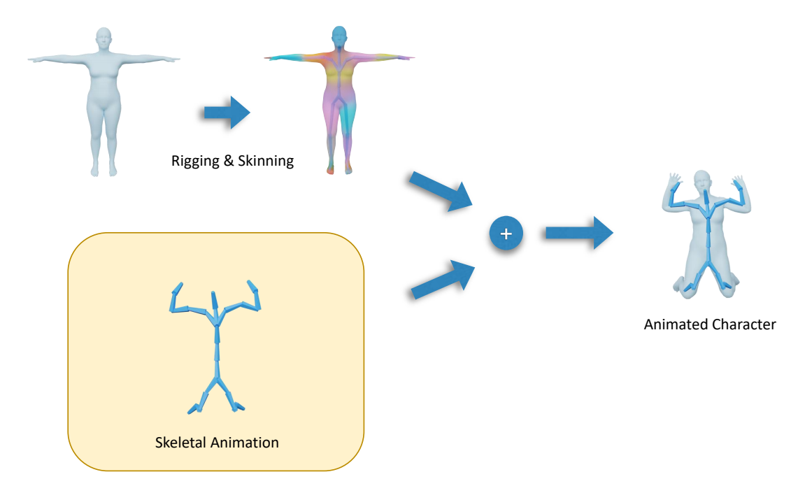
绑定与蒙皮概念
✅ Rigging:创建脸部控制器或身体骨骼。黄色为在 Mesh 顶点内放置的骨骼。
✅ Sinning:让控制器带动皮肤运动。或让 Mesh 顶点跟着骨骼运动。
骨骼代理的角色驱动的局限性
- 非刚性形变:
- LBS(线性混合蒙皮)无法表达肌肉膨胀、软组织形变
- 解决方案:PartMM(Part-aware Mixture Model)替代LBS
- 高频细节丢失:
- 骨骼代理只能捕获低频运动(关节旋转)
- 解决方案:法线修正、位移残差学习
P12
Skinning Deformation
计算方式一

✅ 骨骼运动的旋转和平移分别为 \(R\) 和 \(t\),关节的位置和朝向则变成了 \({Q}'\) 和 \({o}'\).
✅ 求 \(x\) 的新位置 \({x}'\). 本质上就是坐标系变换:世界坐标系 → \({o}\) 坐标系 → \({o}'\) 坐标系 → 世界坐标系
P13
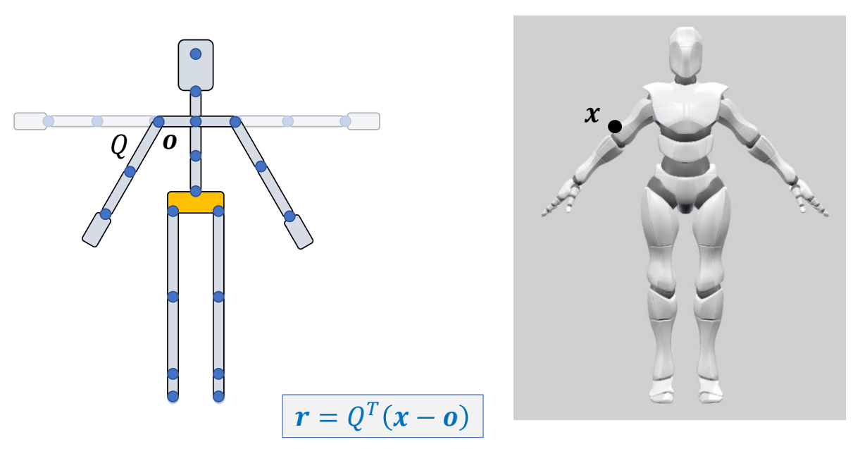
计算方式二
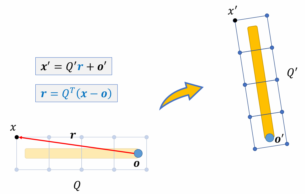
✅ \(r\) 为 \(x\) 在骨骼坐标的表达,用 \(r\) 计算更简洁。
P16
Bind Pose
✅ 当骨骼参考姿态与 Mesh 参考姿态不一致时,需要先旋转骨骼到 Mesh 姿态。
P20
Skinning Deformation - 2 joints
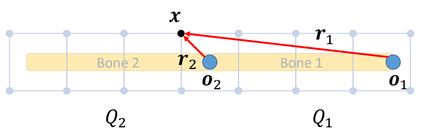
$$ r_2=Q^T_2(x-o_2) \quad \quad r_1=Q^T_1(x-o_1) $$
✅ 多骨骼场景,\(x\) 在关节 \(O_1\) 和 \(O_2\) 下分别 \(r_1\) 和 \(r_2\) 两种表达。
P23

✅ 得到的旋转后表达分别为 \({x}'_1\) 和 \({x}'_2\),通过权重对它们结合。
P29
✅ 同时考虑所有 Mesh 顶点和所有关节。
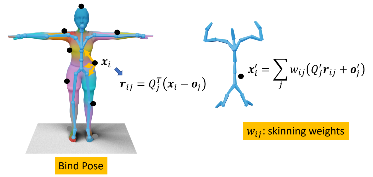
补充:LBS 基础(
LBS 是最流行的角色蒙皮方法。它的核心公式:
$$ \mathbf{v} _{i} ^{t} = \sum _{j=1}^{|B|} w _{ij} \left( \mathbf{R} _{j} ^{t} \mathbf{p} _{i} + \mathbf{T} _{j} ^{t} \right) $$
| 符号 | 含义 | 通俗解释 |
|---|---|---|
| \(\mathbf{v} _{i} ^{t}\) | 第 \(t\) 个姿态中第 \(i\) 个顶点的位置 | 动画中某一帧的某个表面点 |
| \(\mathbf{p} _{i}\) | 静止姿态中第 \(i\) 个顶点的位置 | 角色摆好标准姿势时的那个点 |
| \(w _{ij}\) | 第 \(j\) 根骨头对第 \(i\) 个顶点的影响权重 | 这根骨头对这个点有多大的控制力 |
| \(\mathbf{R} _{j} ^{t}\) | 第 \(t\) 个姿态中第 \(j\) 根骨头的旋转矩阵 | 这根骨头转了多少 |
| \(\mathbf{T} _{j} ^{t}\) | 第 \(t\) 个姿态中第 \(j\) 根骨头的平移向量 | 这根骨头平移了多少 |
| \( | B | \) |
通俗理解:
想象你有一块橡皮泥(顶点),它被钉在几根棍子(骨头)上。
每根棍子上都有一个钉子,钉子对橡皮泥的拉力就是权重 w。

当棍子移动时,橡皮泥的位置 = 每根棍子拉力 × 棍子移动距离 的总和
LBS 权重的约束条件
为了让 LBS 模型有意义,权重 \(w _{ij}\) 需要满足三个条件:
-
非负性(Non-negativity):\(w _{ij} \geq 0\)
- 骨头不能"推"顶点,只能"拉"
-
凸性/仿射性(Affinity):\(\sum _{j=1}^{|B|} w _{ij} = 1\)
- 所有骨头对一个顶点的总影响权重等于 1
- 这保证了如果所有骨头都不动,顶点也不动
-
稀疏性(Sparseness):\(|\{w _{ij} | w _{ij} \neq 0\}| \leq |K|\)
- 每个顶点最多被 \(|K|\) 根骨头影响
- 在实际应用中,通常 \(|K| = 4\)(称为 4-bone skinning)
- 这是为了 GPU 加速——每个顶点只需计算 4 个变换
刚性骨骼约束
旋转矩阵 \(\mathbf{R} _{j} ^{t}\) 必须满足正交约束:
$$ \mathbf{R} _{j} ^{t} {}^{T} \mathbf{R} _{j} ^{t} = \mathbf{I}, \quad \det(\mathbf{R} _{j} ^{t}) = 1 $$
通俗理解:
"刚性"意味着骨头不能被拉伸、压缩或剪切。
旋转只会改变方向,不会改变长度。

对比:
- 刚性旋转:把一本书转个角度,书还是原来的形状
- 非刚性变换:把一本书拉长、压扁、撕扯——这些都不允许
P31
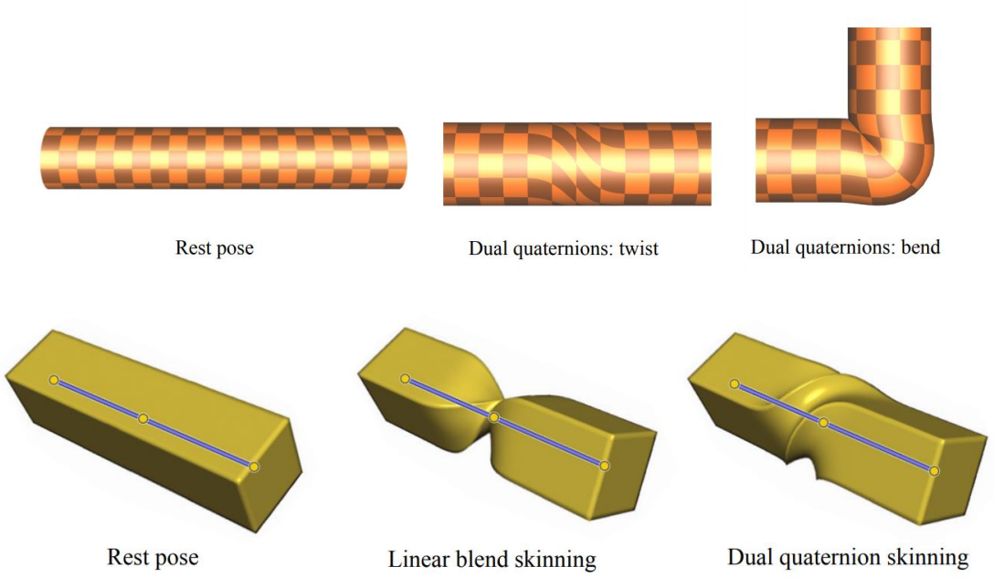
Linear Blend Skinning (LBS)
$$ {x}'_ i= \sum_ {j=1} ^ {m} w _ {ij}({Q}'_ jr_{ij}+{o}'_j) $$
- Used widely in industry
- Efficient and GPU-friendly
- Games like it
✅ Bind Pose:让骨骼与 Mesh 对齐,为 Bind Pose.
✅ Bind Pose 情况下 Motion 不一定为零。
P33
Automatic Skinning?
 |
 |
Pinocchio [Baran et al., 2007]
P37
Linear Blend Skinning (LBS)

✅ 公式第一项对 \(R_j\) 所加权,所得到的很有可能不再是旋转矩阵。
存在的问题: Candy-Wrapper Artifact
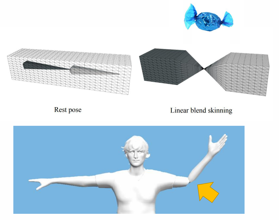
P40
Advanced Skinning Methods
-
Multi-linear Skinning (we will not cover this)
- Multi-weight enveloping [Wang and Phillips 2002]
- Animation Space [Merry et al. 2006]
- ……
-
Nonlinear Skinning
- Dual-quaternion Skinning (DQS)
- Skelebones (PartMM) — GaussiAnimate (ReadPapers/220): 用 Part-aware Mixture Model 替代 LBS。核心:(1) 用空间距离 softmax 计算 part affinity 概率替代人工皮肤权重;(2) 用 MLP 学习的非线性残差 \(x + \Delta T_j(x)\) 替代刚体变换,突破 LBS 线性上限,PSNR 比 LBS 高 17.3%。原本用于 3DGS 驱动,理论上也可用于 Mesh 驱动,但 Mesh 场景下面临三个问题:(1) MLP 推理比 LBS 矩阵乘法慢,不利于实时渲染;(2) MLP 输出可能跨帧跳跃,时间一致性不如 LBS 稳定;(3) 现有引擎全基于 LBS/DQS 构建,替换绑定方案工程成本高。Mesh 本身有拓扑约束兜底,LBS/DQS/SSD 已足够;PartMM 对没有拓扑的 3DGS 价值更大。
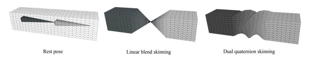
✅ DQ:对偶四元数。
P41
Non-linear Skinning
quaternions and SLERP
Can we use quaternions and SLERP?
P42
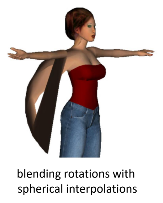
✅ 不行。原因:第一项与第二项必须要配合好,否则会乱掉。
P43
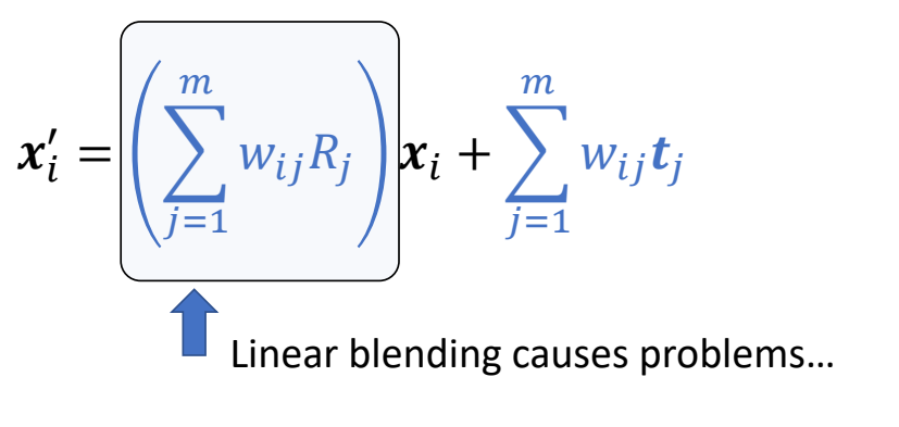
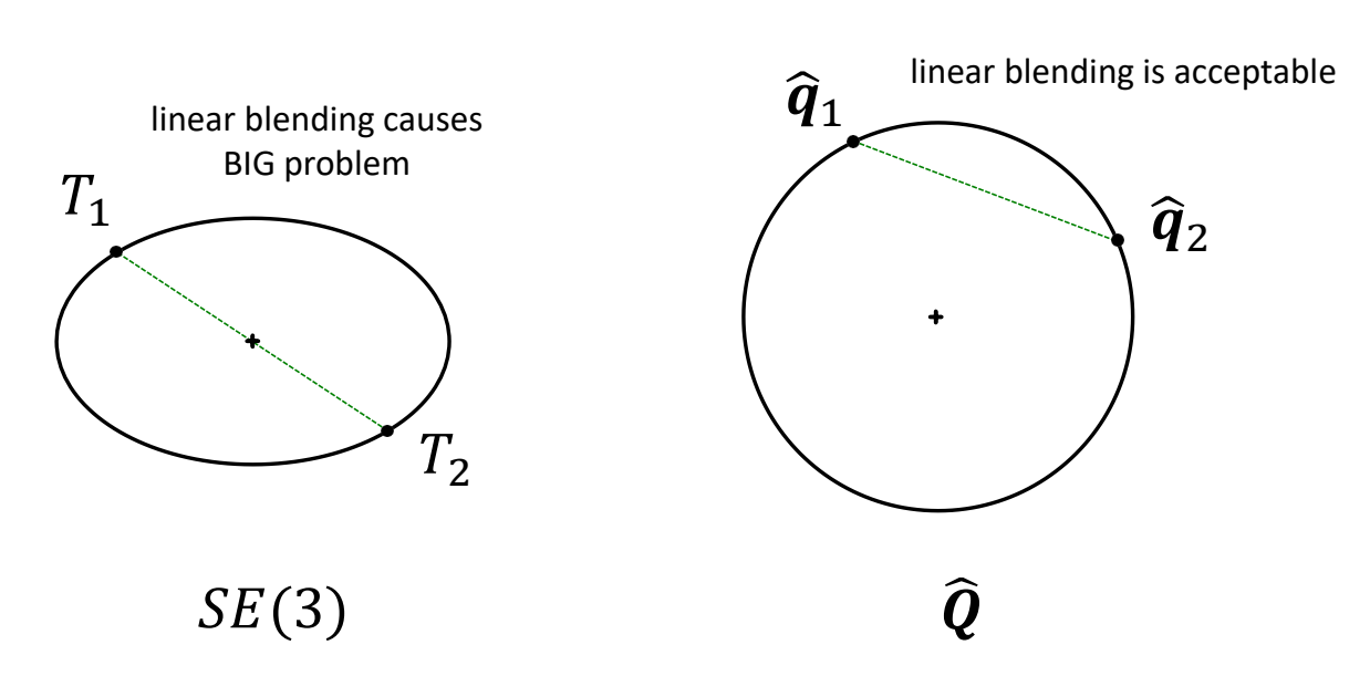
从公式角度来解释不行的原因
$$ {x}' _ i = ( \sum _ {j=1}^{m} w _ {ij} R _ j) x _ i+ \sum _ {j=1}^{m}w _ {ij}t_ j $$
$$ R \in SO(3) $$
$$ T_j=\begin{bmatrix} R_j & t_j\\ 0 &1 \end{bmatrix} \in SE(3) $$
✅ \(T_j\) 构成一个刚性变换群。
P46
Interpolation in 𝑆𝑂(3)
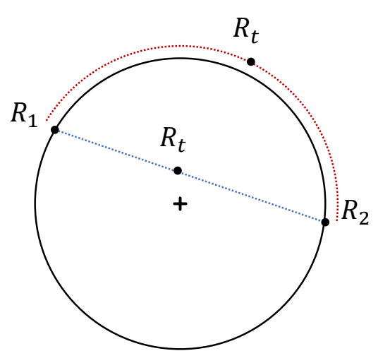
✅ 线性插值和 SLERP 插值 SO(3) 上。
P49
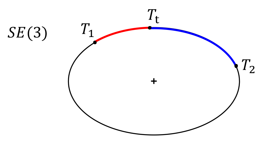
Interpolation in 𝑆𝐸(3)
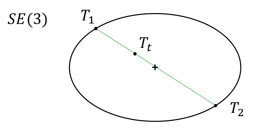
✅ SE(3)上的线性插值,插值到一个退化的点。
P51
Intrinsic Blending
P52
Dual-Quaternion Skinning (DQS)
- Approximation of intrinsic averages in SE(3)
Ladislav Kavan, Steven Collins, Jiri Zara, Carol O‘Sullivan. Geometric Skinning with
Approximate Dual Quaternion Blending, ACM Transaction on Graphics, 27(4), 2008.
✅ 把旋转 + 平移的刚性变换表达为对偶四元数。
P54
Dual Numbers
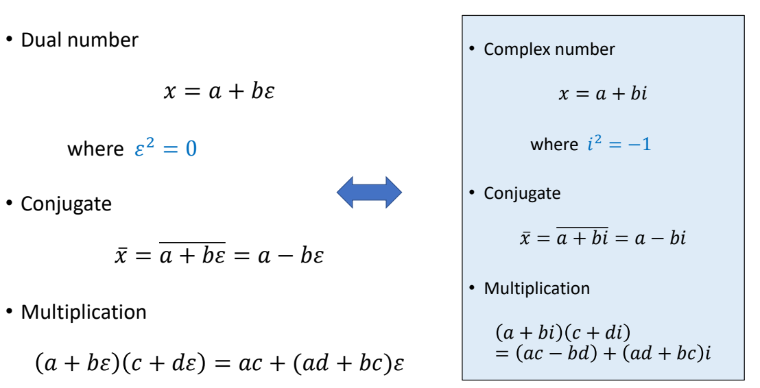
P55
Dual Quaternion
- Dual quaternion
$$ \hat{q} =q_0 + \varepsilon q_\varepsilon $$
$$ \text{where } \varepsilon^2=0 $$
A good note of dual-quaternion:
https://faculty.sites.iastate.edu/jia/files/inline-files/dual-quaternion.pdf
P56
Dual Quaternion
- Scalar Multiplication
$$ s\hat{q}=sq_r+sq_\varepsilon\varepsilon $$
- Addition
$$ \hat{q} _ 1 + \hat{q} _2=q _ {r1}+ q _ {r2} + \varepsilon (q _ {\varepsilon 1} + q _ {\varepsilon 2}) $$
- Multiplication
$$ \hat{q} _ 1 \hat{q} _ 2 = q _ {r1} q _ {r2} + \varepsilon (q _ {r1} q _ {\varepsilon 2} + q _ {r2} q _ {\varepsilon 1}) $$
P57
Dual Quaternion
- Dual quaternion
$$ \hat{q}=q_0+\varepsilon q_\varepsilon $$
- Conjugation
$$ \mathrm{I}:\hat{q}^* =q ^ * _ 0+\varepsilon q ^ * _ \varepsilon $$
$$ \mathrm{II}:\hat{q}^ {\circ} =q _ 0 - \varepsilon q _ \varepsilon $$
$$ \mathrm{III}: \hat{q} ^ \star = q ^ * _ 0 - \varepsilon q ^ *_ \varepsilon $$
$$ \quad \quad \quad \quad = ({\hat{q} ^ *}) ^ {\circ} = (\hat{q} ^ {\circ}) ^ * $$
$$ (\hat{q} _1\hat{q}_2)^\times =\hat{q} _1 ^\times \hat{q}_2^\times $$
- Norm
$$ ||\hat{q}||=\sqrt{\hat{q}^*\hat{q}} =||q_0||+\frac{\varepsilon (q_0\cdot q_\varepsilon) }{||q_0||} $$
P58
Dual Quaternion
- Unit dual quaternion: \(||\hat{q}||=1\), which requires:
$$ ||q_0||=1 $$
$$ q_0 \cdot q_\varepsilon=0 $$
P59
Dual Quaternion ⇔ Rigid Transformation
- Like quaternion, any rigid transformation \(T \in SE(3)\) can be converted into a unit dual quaternion
$$ Tx=Rx+t $$
$$ T=[R\mid t]\to \hat{q} =q_0+\varepsilon q_\varepsilon $$
$$ \begin{matrix} q_0=r \quad & \text{ quaternion of } R \quad \quad\quad\quad\\ q_\varepsilon =\frac{1}{2} tr & \text{ pure quaternion } t = (0,t) \end{matrix} $$
✅ 把一个刚性变换表示为对偶四元数。
P60
Dual Quaternion ⇔ Rigid Transformation
- Transform a vector \(v\) using unit dual quaternion
$$ {\hat{v} }' =\hat{q} \hat{v} \hat{q} ^\star $$
where
$$ \begin{align*} \hat{v} & = 1+\varepsilon (0,v) \\ & =(1,0,0,0)+\varepsilon (0,v_x,v_y,v_z) \end{align*} $$
$$ \quad $$
$$ \mathrm{III}: \hat{q} ^ \star = q ^ * _ 0 - \varepsilon q ^ *_ \varepsilon $$
$$ \quad \quad \quad \quad = ({\hat{q} ^ *}) ^ {\circ} = (\hat{q} ^ {\circ}) ^ * $$
P61
Dual Quaternion ⇔ Rigid Transformation
- Like quaternion, any rigid transformation \(T \in SE(3)\) can be converted into a unit dual quaternion
$$ T=[R\mid t]\to \hat{q} =q_0+\varepsilon q_\varepsilon $$
$$ \begin{matrix} q_0=r \quad \\ q_\varepsilon =\frac{1}{2} tr \end{matrix} $$
\(\hat{q}\) and \(-\hat{q}\) represent the same transformation \(\hat{Q}\) is a double cover of \(SE(3)\)
P62
Double Cover Visualized
P63
Interpolating Dual-Quaternion
P64
Dual-Quaternion Linear Blending (DLB)

P65
Dual-Quaternion Skinning (DQS)
P66
Budging Artifact of DQS
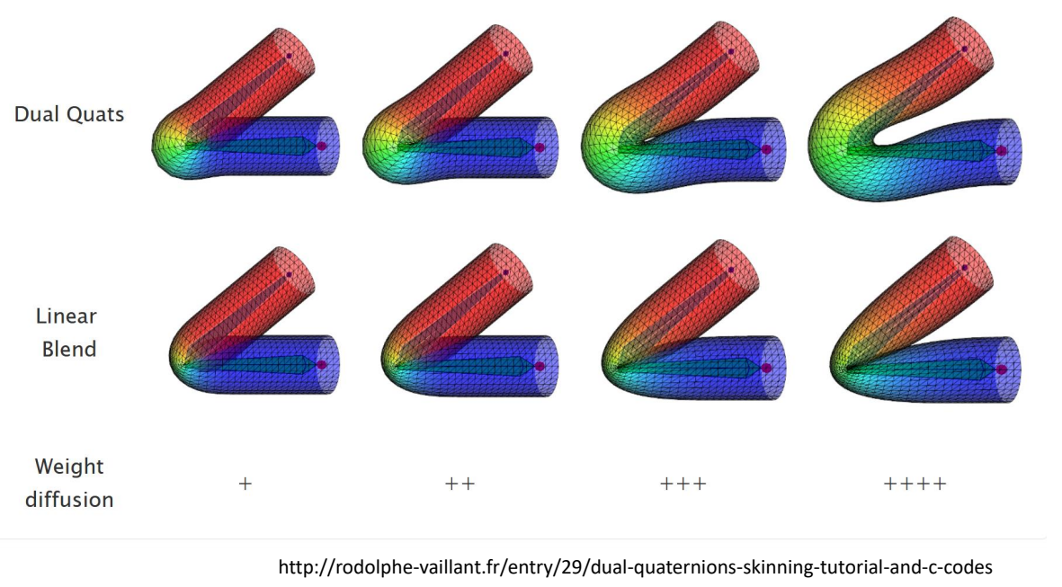
✅ 越往右蒙皮权重越光滑。
✅ DQBS 也有比较严重的 artifacts.
P67
How to Correct LBS?
✅ LBS 的天然缺陷
P69
How to Correct LBS?
P74
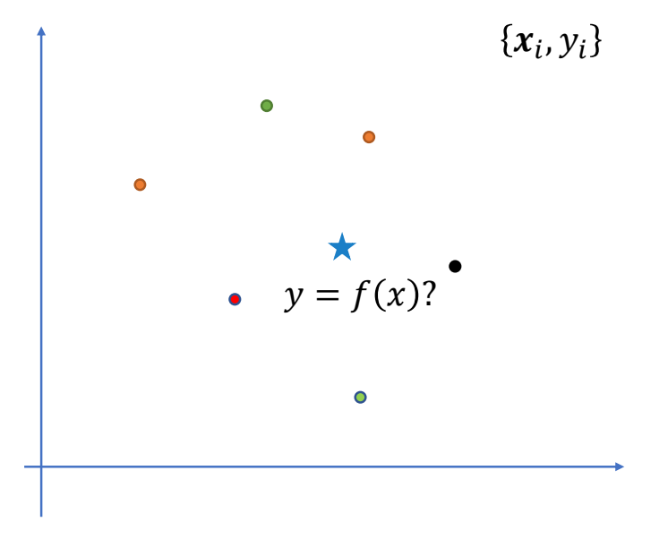
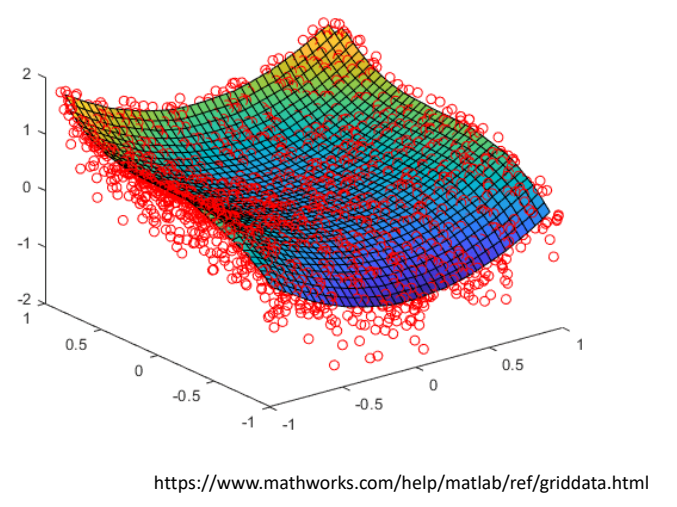
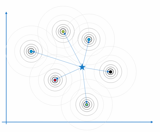
Scattered Data Interpolation
P76
Scattered Data Interpolation
- Linear
- Least squares
- Splines
- Inverse distance weighting
- Gaussian process
- Radial Basis Function
- ……
P81
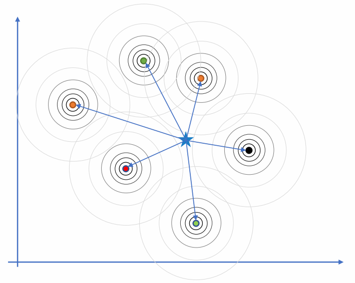
Radial Basis Function (RBF) Interpolation
$$ y=\sum_{i=1}^{k} w_i\varphi (||x-x_i||) $$
P83
Radial Basis Function (RBF) Interpolation
$$ y=\sum_{i=1}^{k} w_i\varphi (||x-x_i||) $$
How to compute \(w_i\) ? We need \(f(x_i)=y_i\)
$$
\begin{bmatrix}
R_{1,1} & R_{1,2} & \cdots & R_{1,K} \\
R_{2,1} & R_{2,2} & & \vdots \\
\vdots & & \ddots & \vdots \\
R_{K,1} & \cdots & \cdots & R_{K,K}
\end{bmatrix} \begin{bmatrix}
w_1\\
w_2 \\
\vdots\\
w_K
\end{bmatrix}=\begin{bmatrix}
y_1\\
y_2 \\
\vdots\\
y_K
\end{bmatrix}
$$
$$ R_{i,j}=\varphi (||x_i-x_j||) $$
P84
Radial Basis Function (RBF)
$$ y=\sum_{i=1}^{k} w_i\varphi (||x-x_i||) $$
- Gaussian:
$$ \varphi (r)=e^{-(r/c)^2} $$
- Inverse multiquadric:
$$ \varphi (r)=\frac{1}{\sqrt{r^2+c^2} } $$
- Thin plate spline:
$$
\varphi (r)=r^2 \log r
$$
- Polyharmonic splines:
$$
\varphi (r)=\begin{cases}
r^k,k=2n+1\\
\\
r^k \log r,k=2n
\end{cases}
$$
P85
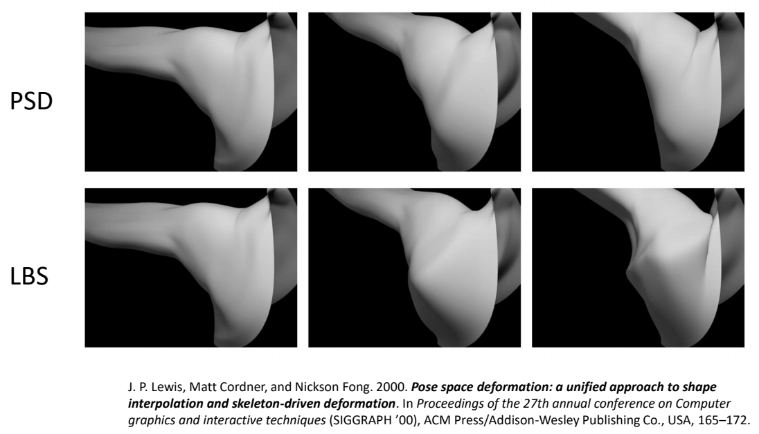
Pose Space Deformation
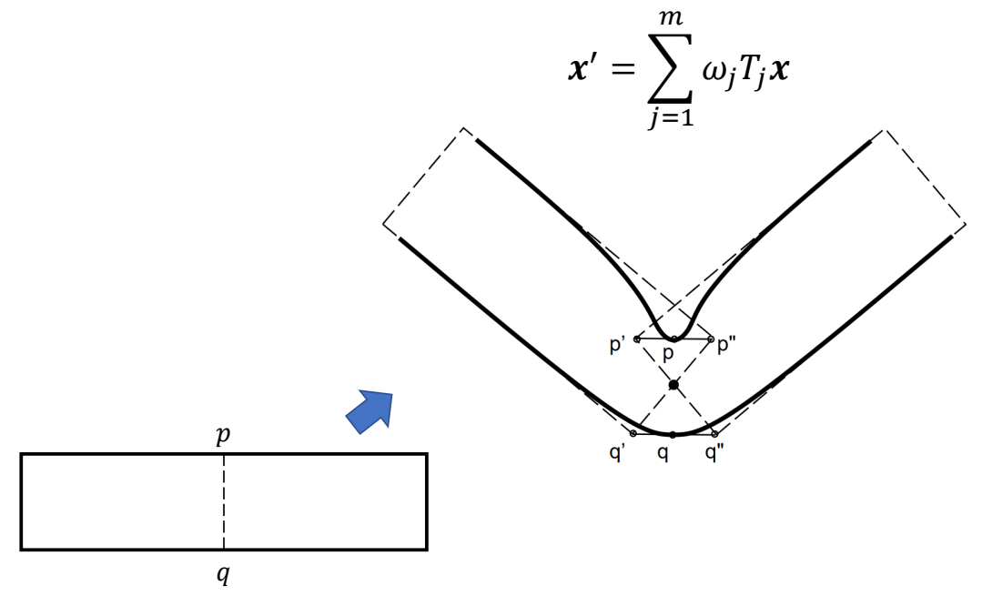
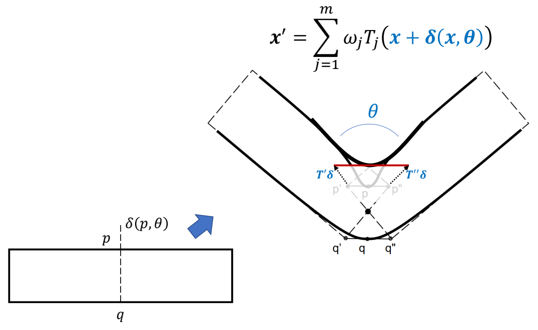
$$ {x}' =\sum_{j=1}^{m} w_iT_j (x+\delta (x,\theta )) $$
- \({x}'= SKIN(PSD(x))\)
- 𝑃𝑆𝐷 is implemented as RBF interpolation
- Example shapes can be created manually
- Or by 3D scanning real people → the SMPL model
J. P. Lewis, Matt Cordner, and Nickson Fong. 2000. Pose space deformation: a unified approach to shape
interpolation and skeleton-driven deformation. In Proceedings of the 27th annual conference on Computer
graphics and interactive techniques (SIGGRAPH ’00), ACM Press/Addison-Wesley Publishing Co., USA, 165–172.
P86
Pose Space Deformation
P87
Issues
- Per-shape or per-vertex interpolation
- Should we interpolate a shape as a whole?
- Local or global interpolation?
- Should a vertex be affected by all joints?
- Interpolation algorithm?
- Is RBF the only choice?
SIGGRAPH Course 2014 — Skinning: Real-time Shape Deformation
P88
Example-based Skinning (EBS) vs. Skeleton Subspace Deformation (SSD)
\(^\ast \)EBS: PSD
\(\quad\)
- Good: Easy to control
- Good: Good quality
- Good: Pose-dependent details (e.g. bulging muscle and extruding veins)
\(\quad\)
- Bad: Creating examples can be cumbersome
- Bad: Extra storage for examples
- Bad: Interpolation needs careful tuning
\(\quad\)
\(^\ast \)SSD: LBS, DQS, etc.
\(\quad\)
- Good: Easy to implement
- Good: Fast and GPU friendly
\(\quad\)
- Bad: Various artifacts
- Bad: Skinning weights needs careful tuning
- Bad: Hard to create pose-dependent details
P89
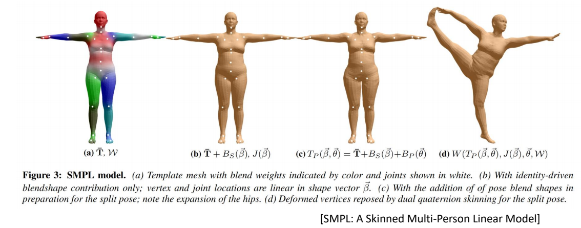
Example: SMPL Model
- A widely adopted human model in ML/CV
- Learned on real scan data
- Combines SSD and EBS techniques
P92
Recall: Principal Component Analysis (PCA)
- Given a dataset {\(x_i\)}, \(x_i \in \mathbb{R} ^N\), then PCA gives
$$ x_i=\bar{x}+\sum_{k=1}^{n} w_{i,k}u_k $$
- \(u_k\) is the \(k\)-th principal component
- A direction in \( \mathbb{R} ^N\) along which the rojection of {\(x_i\)} has the \(k\)-th maximal variance
- \(w_{i,k}=(x_i-\bar{x})\cdot u_k\) is the score of \(x_i\) on \(u_k\)
P93
Recall: Principal Component Analysis (PCA)
• Given a dataset {\(x_i\)}, \(x_i \in \mathbb{R} ^N\), the PCA can be computed by apply eigen decomposition on the covariance matrix
$$ \sum =X^TX=U\begin{bmatrix} \sigma ^2_1 & & & \\ & \sigma ^2_2 & & \\ & & \ddots & \\ & & \sigma ^2_N \end{bmatrix}U^T $$
-
\(X=[x_0-\bar{x}, x_1-\bar{x},\dots ,x_N-\bar{x}]^T\)
-
\(\sigma _i\ge \sigma _j\ge 0\) when \(i< j\), corresponds to the Explained Variance
-
\(U=[u_1,u_2,\dots,u_N]\)
P94
PCA over Body Shapes
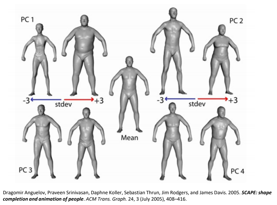
P95
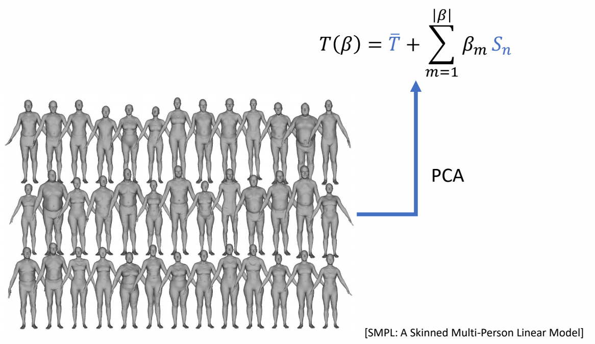
SMPL Model: Body Shape
P96
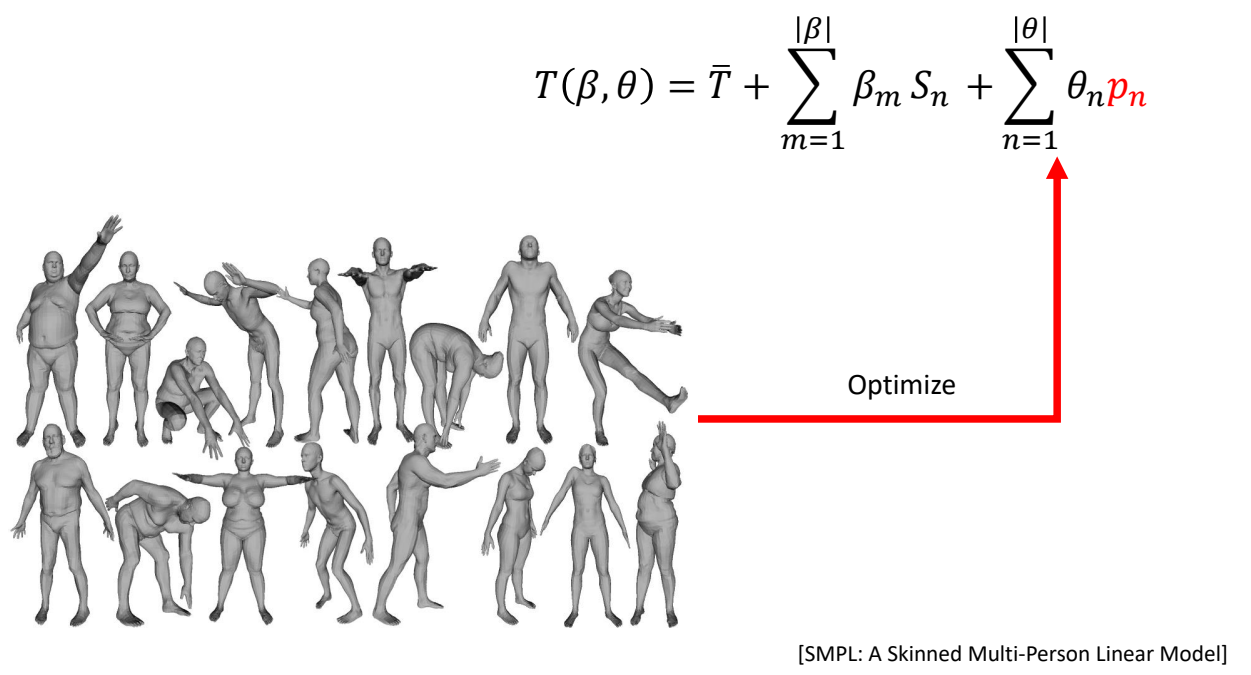
SMPL Model: Pose Blend Shapes
P97
SMPL Model: Deformation
$$ T(\beta ,\theta )=\bar{T} + \sum _ {m=1}^{|\beta |} \beta _ m S_ n + \sum _ {n=1}^{|\theta |}\theta _np_n $$
$$ x=SKIN(T(\beta ,\theta ),\theta ,w) $$
$$ SKIN:\text{LBS, DQS, etc}\dots $$
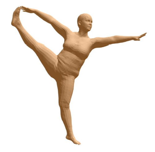
[SMPL: A Skinned Multi-Person Linear Model]
P99
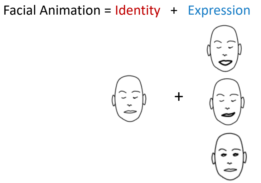
Facial Animation
P101
Facial Animation
✅ \(B_j\) 与 ID 无关,能做出差不多的效果。
✅ 要更精细的效果,可以定义与 ID 相关的 \(B_j\).
P102
Facial Blendshapes
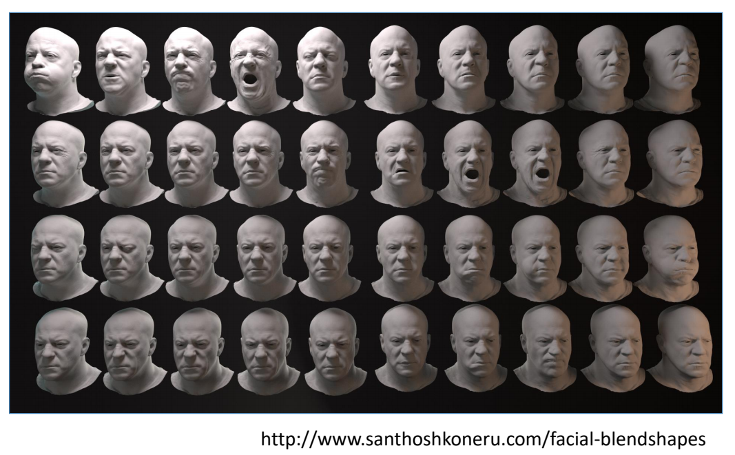
P103
A Typical Set of Blendshapes (ARKit)

P104
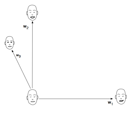
Blendshapes vs. Example-based Skinning
✅ 几种不同的表情基混合方式。
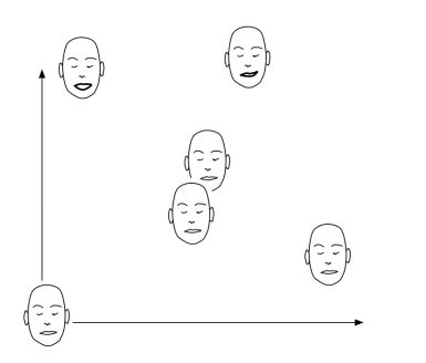
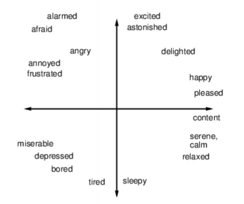
✅ 第二种,直接在几个脸之间做混合,适用于数据少的情况。
P105
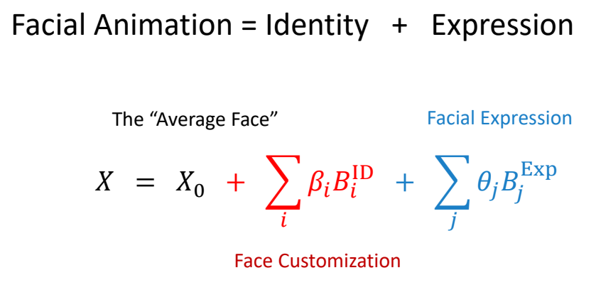
Morphable Face Models
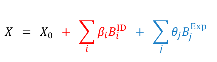
Egger et al. 2020. 3D Morphable Face Models - Past, Present, and Future. ACM Trans. Graph. 39, 5 (June 2020), 157:1-157:38.
✅ 第一项:平均脸。第二项:PCA. 第三项:表情基。
✅ \(B_i^{ID}\) 通常由 PCA 得到。
✅ 基于脸部肌肉的物理仿真。
P107
How to Animate a Face?
P110
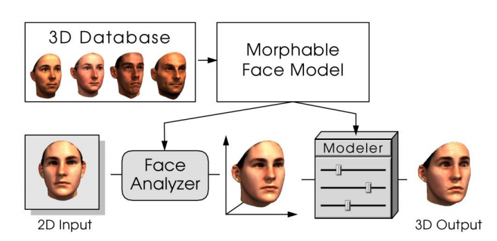
Face Tracking
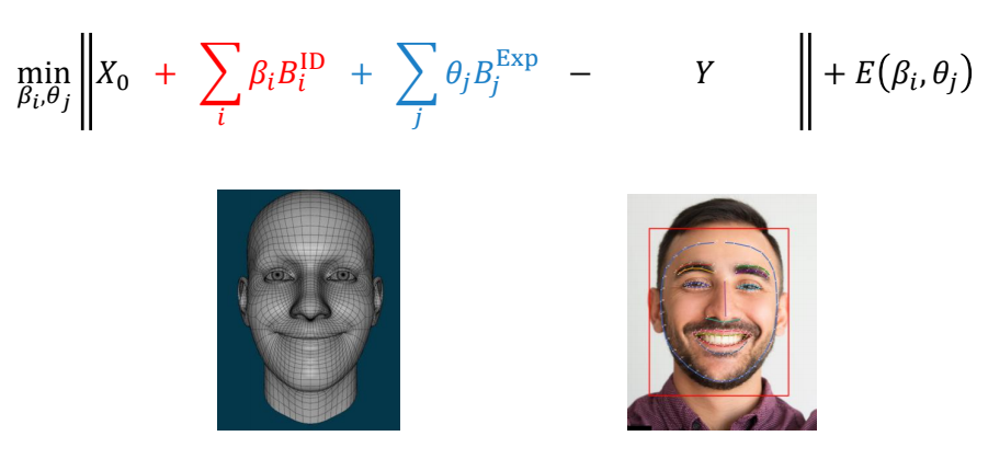
✅ 用一个视频人脸驱动 3D 人脸。
✅ 人脸 \(\overset{①}{\rightarrow} \) 特征点 \(\overset{②}{\rightarrow} \) 表情参数
✅ 1、提取 \(\quad\) 2、IK.
ReadPapers 蒙皮绑定相关论文索引
以下论文收录于 ReadPapers 项目,按核心程度分组。
核心蒙皮 / 绑定论文
| 论文 ID | 论文标题 | 发表 | 蒙皮方法 | 一句话总结 |
|---|---|---|---|---|
| 235 | Smooth Skinning Decomposition with Rigid Bones (SSDR) | SIGGRAPH Asia 2012 | LBS 逆问题 | 从示例姿态反推 LBS 权重和刚性骨骼变换,所有约束作为硬约束严格满足,块坐标下降 + 闭式 SVD 求解,比 LM 快 50-70× |
| 236 | Robust and Accurate Skeletal Rigging from Mesh Sequences | SIGGRAPH 2014 | 全自动绑定 | 从网格序列自动生成骨骼系统:运动驱动聚类 → MST 拓扑重建 → 迭代绑定(权重/关节/变换交替优化)+ 骨骼剪枝 |
基于 LBS 扩展的新表示方法
| 论文 ID | 论文标题 | 发表 | 蒙皮方法 | 一句话总结 |
|---|---|---|---|---|
| 220 | GaussiAnimate: Reconstruct and Rig Animatable Categories with Level of Dynamics | arXiv 2026 | Skelebones (骨架-骨骼脚手架) + PartMM | 从 235/236 取 LBG-VQ 聚类 + SSDR 生成外层 Bones,原创 MCS 骨架化 + 关节检测生成内层 Skeleton,PartMM 非参数化运动匹配解决骨架→骨骼绑定 |
| 234 | SC-GS: Sparse-Controlled Gaussian Splatting for Editable Dynamic Scenes | CVPR 2024 | LBS + 稀疏控制点 | 用 ~512 个稀疏控制点的 6DoF 变换 + LBS 权重插值驱动 ~10 万高斯点,ARAP 正则化保证局部刚性 |
| 225 | TaoAvatar: Real-Time Lifelike Full-Body Talking Avatars for AR via 3DGS | 2025 | SMPL-X++ LBS + 教师-学生蒸馏 | 构建穿衣参数化模板 SMPL-X++,StyleUnet 教师网络学习非刚性变形,蒸馏到轻量 MLP 实现实时 LBS 驱动 |
| 36 | GaussianAvatar: Towards Realistic Human Avatar Modeling from a Single Video | 2023 | SMPL LBS + 3DGS | 以 SMPL 为 template,每个 Mesh 顶点对应一个高斯球,直接复用 SMPL 的 LBS 蒙皮权重驱动 3D 高斯 |
动物/人脸绑定
| 论文 ID | 论文标题 | 发表 | 蒙皮方法 | 一句话总结 |
|---|---|---|---|---|
| 35 | MagicPony: Learning Articulated 3D Animals in the Wild | 2023 | LBS + DMTet 网格 | 单图重建铰接 3D 动物,隐式神经场转显式网格,用 LBS 驱动动物姿态 |
| 32 | Artemis: Articulated Neural Pets with Appearance and Motion Synthesis | 2023 | 体素级 LBS + NGI | CGI 动物资产的体素绑定与蒙皮,复用 CGI 骨骼和蒙皮权重,LBS 驱动八叉树体素形变 + 神经渲染 |
| 95 | SOAP: Style-Omniscient Animatable Portraits | 2024 | 自适应网格重构 + 骨骼插值 | 从单张肖像生成风格化虚拟形象,通过可微分渲染实现网格重拓扑和骨骼绑定,蒙皮权重由邻接边插值 |
说明:论文 ID 对应 ReadPapers 项目中的编号,点击可跳转至完整笔记。其中 235 (SSDR) 和 236 (Rigging) 是本节内容的直接延伸阅读;220 (GaussiAnimate) 展示了经典 LBS/DQS 思想在 3DGS 新表示中的延续。
本文出自CaterpillarStudyGroup,转载请注明出处。
https://caterpillarstudygroup.github.io/GAMES105_mdbook/
P3
Outline
-
Character Kinematics
- Skeleton and forward Kinematics
-
Inverse Kinematics
- IK as a optimization problem
- Optimization approaches
- Cyclic Coordinate Descent (CCD)
- Jacobian and gradient descent method
- Jacobian inverse method
P4
Character Kinematics
the study of the motion of bodies without reference to mass or force
P8
joint, bone, skeleton
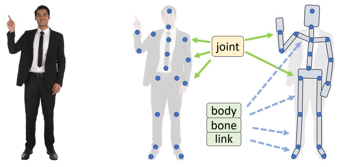
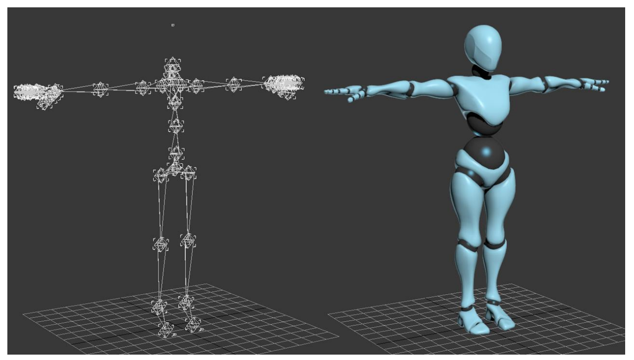
✅ 关注关节的位置和旋转
P13
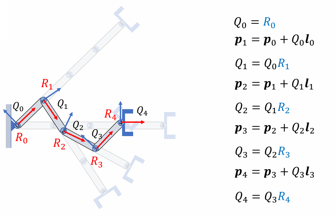
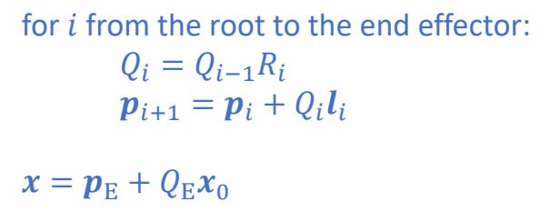
Kinematics of a Chain
问题描述
要使手臂摆成指定的动作,每个关节在各自坐标系下的旋转是多少?

求\(Q_0, Q_1, Q_2, Q_3, Q_4\)
P14
初始pose

$$ Q_0=Q_1=Q_2=Q_3=Q_4=I $$
✅ 这一个定义了5个关节的手臂。在每个关节上绑上一个坐标系。
P15
旋转关节4
把关节4旋转R4以后
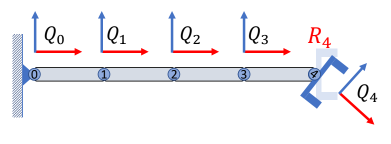
✅ \(Q\):在世界坐标系下的朝向
✅ \(R\):在局部坐标系下的旋转
$$
\begin{matrix}
Q_0=I\quad\\
Q_1=I\quad\\
Q_2=I\quad\\
Q_3=I\quad\\
Q_4={\color{Red}{R_4}}
\end{matrix}
$$
P16
旋转关节3
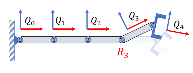
把关节3旋转R3以后,Q3和Q4会同时受到影响
$$
\begin{matrix}
Q_0=I\quad\quad\\
Q_1=I\quad\quad\\
Q_2=I\quad\quad\\
Q_3={\color{Red}{R_3}}\quad\\
Q_4={\color{Red}{R_3}}R_4
\end{matrix}
$$
P17
依次旋转关节2, 1, 0
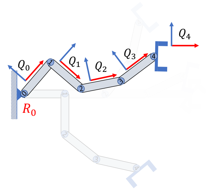
$$ \begin{matrix} Q_0={\color{Red}{R_0}}\quad \quad\quad\quad \\ Q_1={\color{Red}{R_0}}R_1 \quad\quad\quad \\ Q_3={\color{Red}{R_0}}R_1R_2R_3\quad \\ Q_4={\color{Red}{R_0}}R_1R_2R_3R_4 \end{matrix} $$
P20
简化公式,用递推的形式描述

P21
From rotation(local) to orientation(global)
$$ Q_i = Q_{i-1}R_i $$
From orientation(global) to rotation(local)
$$ R_i = Q^T_{i-1}Q_i $$
✅ 这些 \(Q\) 都是全局旋转,\(R\) 是局部旋转。
Kinematics with position
P23
初始状态
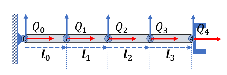
✅ \( 𝒍 \):子关节位置在父坐标系下的坐标。
P31
positon with pose
✅ \(p\) 是全局位置,\( 𝒍 \) 是局部偏移。
P37
Forward Kinematics of a Chain: Summary
position
Given the rotations of all joints \(R_i\), find the coordinates of \(x_0\) in the global frame \(x\):
✅ \(x_0\) 是 \(R_4\) 坐标系下的点,求它在某个父坐标系下的位置。
✅ \(p\):关节在全局坐标系下的位置
✅ 第1步:根据 \(R_i\) 和 \( 𝒍 _i\) 求出 \(Q_i\) 和 \(P_i\)
✅ 第2步:\(E\) 可以是任意父结点,公式都适用
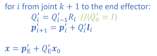
P38
✅ 是上一页的另一种写法,不需提前算出中间变量。
P39
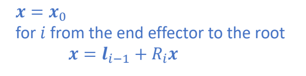
rotation
Given the rotations of all joints \(R_i\), find the coordinates of \(x_0\) relative to the local frame of \(Q_k\):
✅ 已知全局坐标系下的坐标,求 \(Q_k\) 下的坐标。
P40
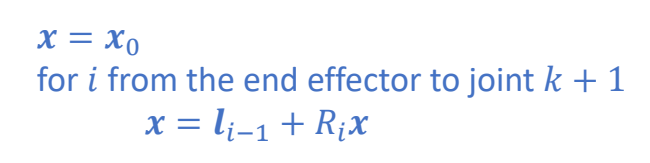
✅ 对应上一页的另一种写法
P41
Kinematics of a Character
骨骼的参数化表示
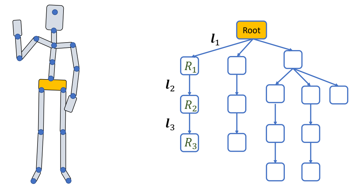
✅ 把角色建模成多条关节链。
P43
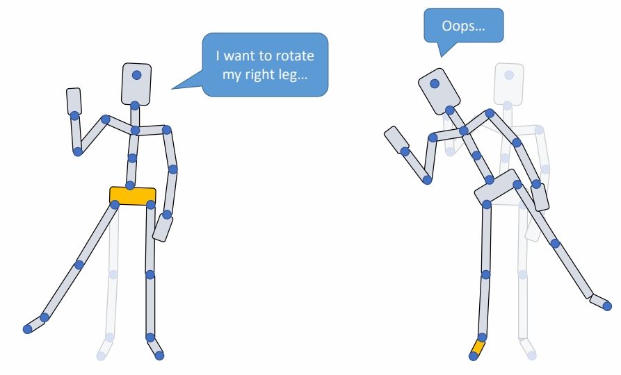
✅ 以不同关节为 root,同样旋转会得到不同效果。
P45
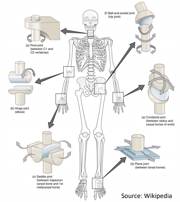
Types of Joints
P50
 | 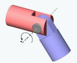 | knee, elbow \({\color{Red}{1 \text{DoF}}}\) \(\theta_{\min }\le \theta\le \theta_{\max } \) hinge joint revolute joint |
 | 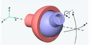 | hip, shoulder \({\color{Red}{3 \text{DoF}}}\) \(\theta_{\min }\preceq \theta \preceq \theta_{\max } \) ball-and-socket joint |
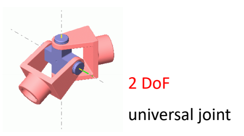 | 手腕。其实手腕不能自转。 2 Dof |
✅ 关节的自由度最多为3,因为不能自主移动。Hips 除外。 ✅ 自由度:一个物理系统,需要多少参数可以唯一准确地描述它的状态。
✅ 6 DOF=3 平移 + 3 旋转。
姿态的参数化表示 Pose Parameters
P55
$$ (t_0,R_0,R_1,R_2\dots \dots ) $$
$$ \text{root } \mid \text{ internal joints} $$
joints are typically in the order that every joint precedes its offspring
for \(i\) in joint_list:
$$ \begin{align*} p_i= & i^,\text{ s parent joint} \\ Q_i=& Q_{pi}R_i \\ x_i= & x_{pi} + Q_{pi}l_i \end{align*} $$
✅ 一个动作的参数化表示:
✅ 全局位置+root 朝向+各关节旋转
✅ 通常要求,关节顺序为父在前子在后,这样只须遍历一遍就能完成 FK.
❓ Q2: how should we allow stretchable bones?
✅ 答:增加参数,3 Dof 增加为 6 Dof.
P58
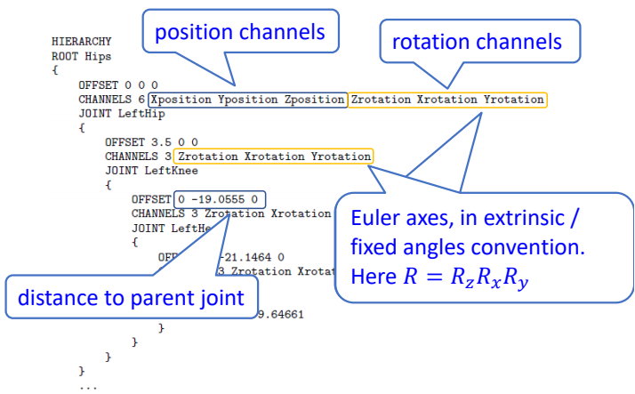
Example: motion data in a file
BVH files
- HIERARCHY: defining T-pose of the character
- MOTION: root position and Euler angles of each joints
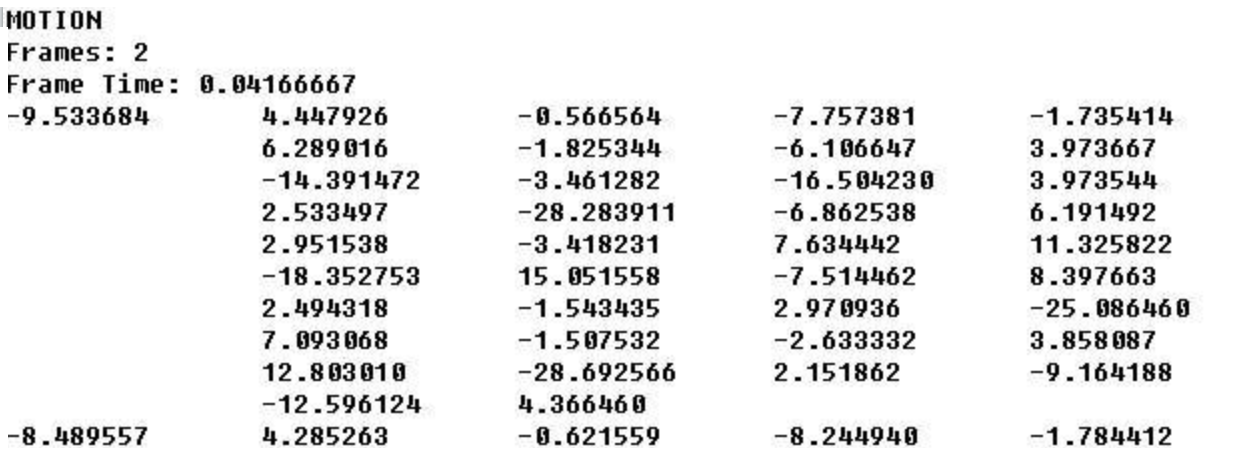
See: https://research.cs.wisc.edu/graphics/Courses/cs-838-1999/Jeff/BVH.html
P59
Inverse Kinematics
🔎 A. Aristidou, J. Lasenby, Y. Chrysanthou, and A. Shamir. 2018.
Inverse Kinematics Techniques in Computer Graphics: A Survey.
Computer Graphics Forum
P61
Forward and Inverse Problems
For a system that can be described by a set of parameters \(\theta \), and a property 𝒙 of the system given by
$$ x=f(\theta ) $$
Forward problem:
-
Given \(\theta \), we need to compute \(x \)
-
Easy to compute since \(f\) is known, the result is unique
-
DoF of \( \theta \) is often much larger than that of \(x \). We cannot easily tune \(\theta \) to achieve a specific value of \(x\).
Inverse problem:
-
Given \(x \), we need to find a set of valid parameters \(\theta \) such that\(x=f(\theta) \)
-
Often need to solve a difficult nonlinear equation, which can have multiple solutions
-
\(x\) is typically meaningful and can be set in intuitive ways
P62
Inverse Kinematics问题描述
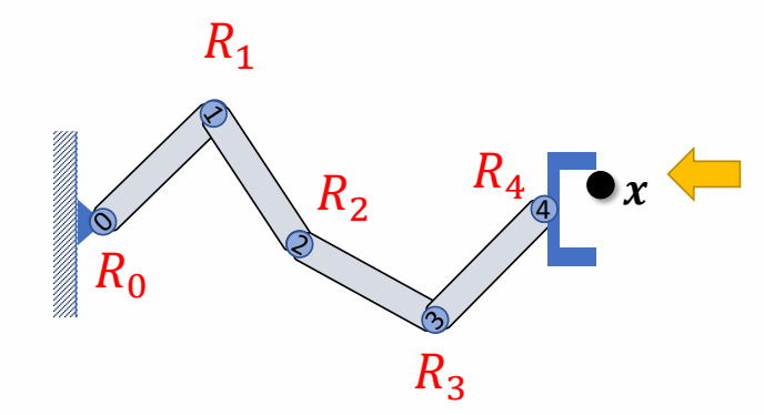
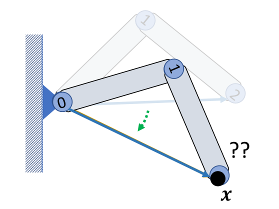
Given the position of the end-effector \(x\), Compute the joint rotations \(R_i\)
P64
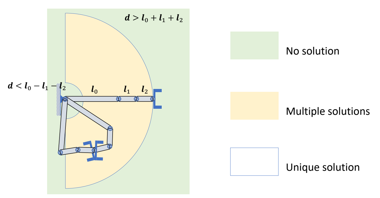
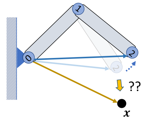
✅ 大部分情况下IK问题是多解问题
P68
two-joint IK
Step 1: Rotate joint 1 such that
$$ ||l_{ox}||=||l_{02}|| $$
✅ 使用余弦公式
Step 2: Rotate joint 0 such that
$$ l_{ox}=l_{02} $$
✅ 叉乘得到旋轴,点乘得到旋转角。
Step 3: Rotate joint 0 around \(l_{ox}\) if necessary
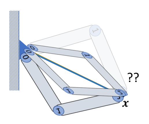
Multi Joint IK
P72
机械臂场景,关节有多个,指定末端结点的位置和朝向
$$ x=f(\theta ) \\ Q=Q(\theta ) $$
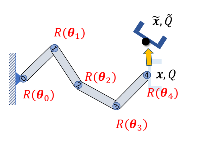
✅ 控制末端点的朝向比较简单,但控制末端点的位置比较难,因此重点考虑如何控制末端点的位置
P74
IK as an Optimization Problem
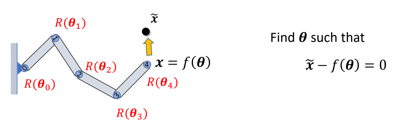
P75
Find \(\theta \) to optimize
$$ \min_{\theta } \frac{1}{2} ||f(\theta )-\tilde{x} ||^2_2 $$
✅ 用迭代的方法,从当前 motion 出发,优化出目标 motion.
P88
CCDIK
Cyclic Coordinate Descent (CCD)
Update parameters along each axis of the coordinate system
Iterate cyclically through all axes

P90
Cyclic Coordinate Descent (CCD) IK
✅ 叉乘得到旋转轴,点乘得到旋转角度。
| Rotate joint 3 such that \(𝒍_{34}\) points towards \(\tilde{x}\) | 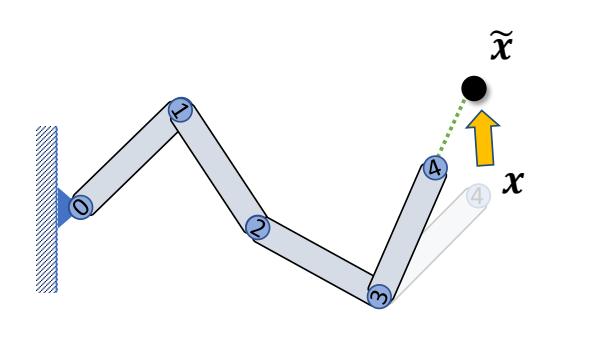 |
| Rotate joint 2 such that \(𝒍_{24}\) points towards \(\tilde{x}\) | 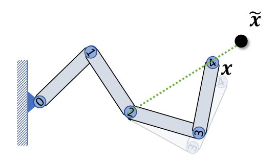 |
| Rotate joint 1 such that \(𝒍_{14}\) points towards \(\tilde{x}\) | 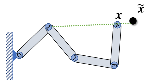 |
| Rotate joint 0 such that \(𝒍_{14}\) points towards \(\tilde{x}\) | 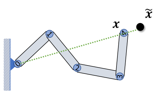 |
| Rotate joint 3 such that \({l}'_{34}\) points towards \(\tilde{x}\) | 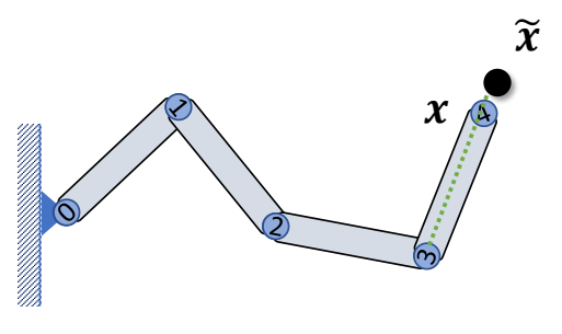 |
| …… |
Iteratively rotation each joint to make the end-effector align with vector between the joint and the target
Easy to implement, very fast
The “first” joint moves more than the others May take many iterations to converge Result can be sensitive to the initial solution
✅ 一个动作序列做 CCD,可能结果不稳定,有跳变。
✅ 前面例子是 3210 的调整顺序,也可以是 0123 的顺序。
✅ 先移到的关节调整幅度会大一点,所以一般从末端开始。
P105
Gradient Descent
CCD下降没有考虑目标函数的性质,考虑目标函数的性质可以得出下降更快的方法。
✅ 关于梯度下降法跳过。
针对目标函数
$$ \min_{\theta } \frac{1}{2} ||f(\theta )-\tilde{x} ||^2_2 $$
其梯度为:
$$
\begin{align*}
\nabla_\theta F(\theta ^i)= & (\frac{\partial f}{\partial \theta }(\theta ^i))^T(f(\theta ^i)-\tilde{x})\\
= & J^T \Delta
\end{align*}
$$
✅ \(J\) 是 Jacobia矩阵, \( \Delta \) 是位置差
P106
因为更新函数为:
$$ \theta ^{i+1}=\theta ^i-\alpha J^T\Delta $$
$$ J= \frac{\partial f}{\partial \theta }=(\frac{\partial f}{\partial \theta_0 }\frac{\partial f}{\partial \theta_1 }\dots \frac{\partial f}{\partial \theta_n } ) $$
J是一个3*N的矩阵,N代表关节数。
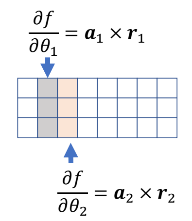
怎么计算J?
方法一:使用machine learning framework的autograd功能
方法二:有限差分
方法三:Geometric Approach
P114
Geometric Approach
问题描述
Assuming all joints are hinge joint
求关节 1 旋转轴 \(a_1\),对 \(x\) 位移的影响
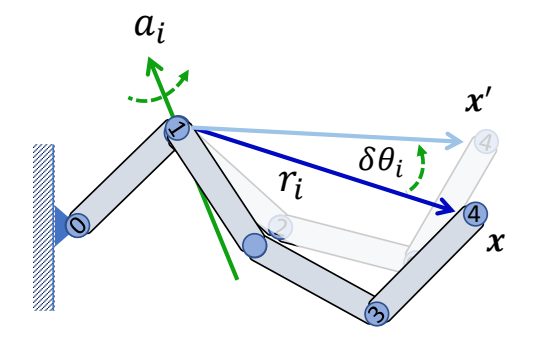
计算过程
$$ {x}' -x=(\sin \delta \theta _i)a_i\times r_i+(1-\cos \delta \theta _i)a_i\times(a_i\times r_i) $$
$$ \frac{ \partial f }{\partial \theta _ i} = \lim _ {\delta \theta _ i \to 0} \frac{{x}'-x }{\delta \theta _ i}= a _ i\times r _i $$
P117
更通用的场景- ball joints
❓ How to deal with ball joints?
A ball joint parameterized as Euler angles:
$$ 𝑅_𝑖 = 𝑅_{𝑖𝑥}𝑅_{𝑖𝑦}𝑅_{𝑖𝑧} $$
can be considered as a compound joint with three hinge joints
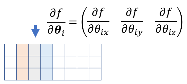
✅ 一个ball joint可以看作是3个hint joint。因此占J矩阵的3列。
也可以写成这种形式:
$$ \frac{ \partial f }{\partial \theta _ {i\ast } } = a _ {i\ast } \times r _ i $$
f对某一个欧拉角的导数,等于这个欧拉角的轴叉乘上末端点到关节点的距离。
需要注意的是,这个的旋转轴a是在世界坐标系下的表示,因此要有一个坐标系的转换。
$$ \begin{align*} 𝒂_{𝑖𝑥} & =𝑄_{𝑖−1}𝒆_𝑥 \\ 𝒂_{𝑖𝑦}& = 𝑄_{𝑖−1}𝑅_{𝑖𝑥}𝒆_𝑦\\ 𝒂_{𝑖𝑧} &= 𝑄_{𝑖−1}𝑅_{𝑖𝑥}𝑅_{𝑖𝑦}𝒆_𝑧 \end{align*} $$
❓ 问:Can we parameterize a ball joint using axis-angle \(\theta u\) and compute Jacobian as
$$ \begin{matrix} \frac{\partial f}{\partial \theta _i} =\theta u\times r_i & ??? \end{matrix} $$
✅ 答:不可以。Jacobian for axis-angle representation has a rather complicated formulation…
P121
Jacobian Transpose / Gradient Descent
First-order approach, convergence can be slow Need to re-compute Jacobian at each iteration
✅ 怎么求 \(J\),这里讲了 3 种方法:(1)backward 框架(2)差分(3)几何计算。实际上直接用 1 可以解决,不需要自己去算,因此跳过。
✅ 特点:(1)迭代次数比 CCD 少(2)计算量比 CCD 大。
P122
✅ 数值插值算法见 GAMES102.
P124
Quadratic Programming 二次规划问题
✅ 这几页介绍二次函数求极值的问题。
$$ \min_{\theta } F(\theta )=\frac{1}{2} \theta ^TA\theta +b^T\theta $$
where \(A\) is positive definite:
$$ A=A^T,\theta ^TA\theta \ge 0 \text{ for any } \theta $$
P126
公式直接求解
$$ \begin{matrix} \text{Gradient}: \nabla_\theta F(\theta )=A\theta +b \\ \text{Optimality condition}: \nabla_\theta F(\theta ^\ast )=0\\ {\color{Blue} \Downarrow } \\ \theta ^\ast =-A^{-1}b \end{matrix} $$
✅ 二次函数的极值点可以直接从公式求出来
P127
Gauss-Newton Method
✅ IK问题也可以转化为二次函数求极值的问题
$$ F(\theta )=\frac{1}{2} ||f(\theta )-\tilde{x} ||^2_2 $$
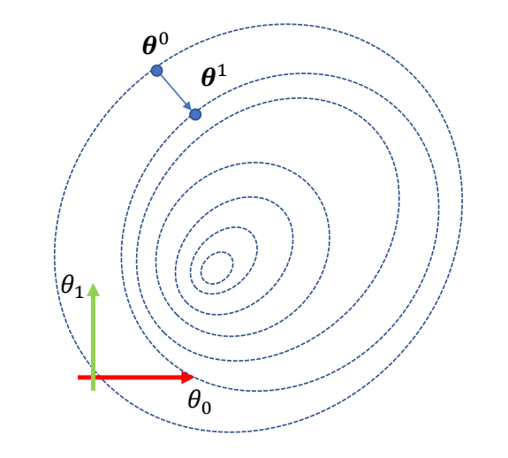
Consider the first-order approximation of \(f(\theta)\) at \(\theta^0\)
✅ 把 \(f(\theta )\) 在 \(\theta ^{\circ} \) 处一阶泰勒展开。
$$ \begin{align*} f(\theta)\approx & f(\theta^0) + \frac{\partial f}{\partial \theta} (\theta^0)(\theta-\theta^0) \\ = & f(\theta^0)+J(\theta-\theta^0) \end{align*} $$
P128
✅ 把它代入目标函数。
\begin{align*} f(\theta)\approx & \frac{1}{2}||f(\theta^0)+J(\theta -\theta ^0)-\tilde{x}||^2_2 \\ = &\frac{1}{2} (\theta -\theta ^0)^TJ^TJ(\theta -\theta ^0)\\ & +(\theta -\theta ^0)^TJ^T(f(\theta ^0)-\tilde{x})+c \end{align*}
P129
first-order optimality condition
✅ 令 \((\nabla F (\theta ))^T=0\)
$$ \begin{matrix} f(\theta)\approx \frac{1}{2}||f(\theta^0)+J(\theta -\theta ^0)-\tilde{x}||^2_2 \\ \Downarrow \\ (\nabla F (\theta ))^T=J^TJ(\theta-\theta^0)+J^T(f(\theta^0)-\tilde{x} )=0 \end{matrix} $$
P133
$$
J^TJ(\theta-\theta^0)=-J^T\Delta
$$
if \(J^TJ\) 不可逆
✅ \(J\) 的维度是 \(3\times N\),因此 \(J^TJ\) 不可逆。
\(J^TJ\) is \({\color{Red} {\text{NOT}}}\) invertible, but \(JJ^T\) can be invertible
P134
因此做以下转化:
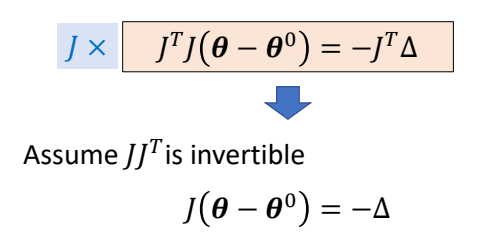
✅ \(\Delta\) 是当前和目标的末端点位置之差。
P135
$$ J(\theta-\theta^0)=\tilde{x} -f(\theta^0) $$
P137
$$ \begin{align*} \theta = & \theta ^0-J^+\Delta \\ = & \theta ^0-J^T(JJ^T)^{-1}\Delta \end{align*} $$
\(J^+\)表示J的(Moore-Penrose) Pseudoinverse
P138
if \(J^TJ\) 可逆
$$ J^TJ(\theta-\theta^0)=-J^T\Delta $$
If \(J^TJ\) is invertible, we have
$$ \theta = \theta^0 - (J^TJ)^{-1}J^T\Delta $$
but when can \(J^TJ\) be invertible?
P141
✅ 答:改变IK的约束条件(例如增加中间关节的位置要求)和自由度(例如限制关节的自由度),可改变 \(J\) 的形状为方阵或高瘦阵,此时 \(J^TJ\) 可逆,则换一种方式求逆。
P143
对比
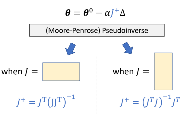
✅ 左:欠约束,右:过约束。
✅ 由于这个方法的本质是把高度非线性的函数做了线性化,所以只是在当前位置附近才有效,远了误差就会非常大。因此增加learning rate。
P145
Usually faster than gradient descent/Jacobian transpose method.
Any problem? \(JJ^T/J^TJ\) can be (near) singular!
✅ 快一点是因为 \(J^+\) 是近似的 \(J\),计算量较小,问题是可能得到一个错很远的 \(J^+\),导致结果不稳定。
P147
Damped Jacobian Inverse Method
✅ 上一页的问题是伪逆\(J^+\) 引入的不稳定。
✅ 解决方法:引 \(\lambda\) 阻尼项
$$ J^\ast =J^T(JJ^T+\lambda I)^{-1} $$
$$ J^\ast =(J^TJ+\lambda I)^{-1}J^T $$
P148
Also called Levenberg-Marquardt algorithm
✅ 引 \(\lambda\) 阻尼顶后,两种方式的计算结果相同。
✅ 当 \(\lambda\) 很大时,此方法等价于梯度下降法。
P149
\(\lambda\) 的几何意义
✅ 相当于正则项 ✅ 进一步地,分别给每个关节移动权重。
✅ 权重越大,移动越小。
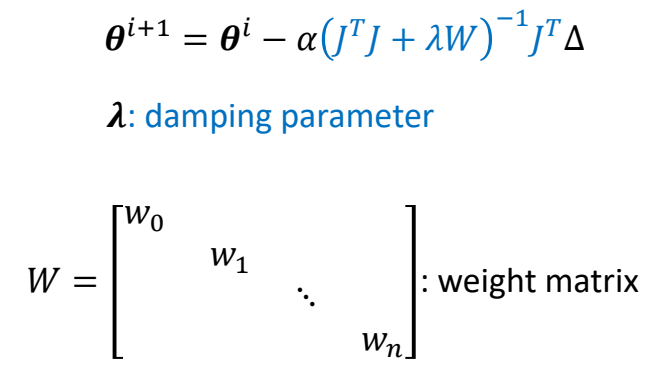
P152
Character 全身IK
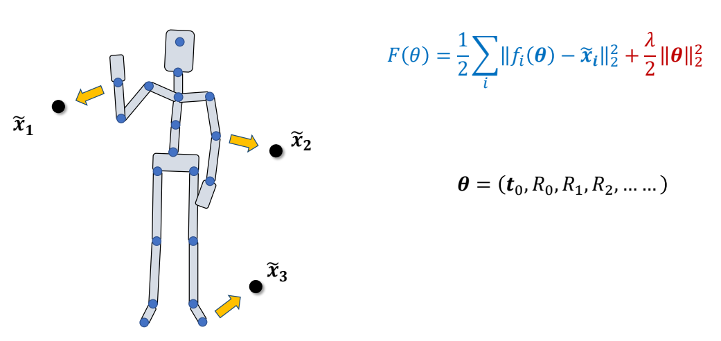
✅ 全身 IK,不同链条上都有目标点。
✅ 可以同时优化所有链,或选一个或选一些。
✅ IK 要更新哪关节也可以自由设定。
P156
总结
✅ IK问题可以使用优化方法,不同优化方法对应不同 IK 方法,例如:
CCD → CCDIK
梯度下降法 → Jacobian transpose
Gaussian → Jacobian Inverse
✅ IK问题可以使用启发式方法,例如FABRIK Andreas Aristidou and Joan Lasenby. 2011.
🔎 FABRIK: A fast, iterative solver for the Inverse Kinematics problem.
Graphical Models
P158
✅ Slerp 结合 Sbline.
✅ 50 fps → 60 fps:先插值,再采样
✅ 惯性插值:UE 基于 SPD 求约束来做 IK
✅ 参考 Darel Holden 博客
本文出自CaterpillarStudyGroup,转载请注明出处。
https://caterpillarstudygroup.github.io/GAMES105_mdbook/
P3
Outline
-
Character Kinematics (cont.)
- Motion Retargeting
- Full-body IK
-
Keyframe Animation
- Interpolation and splines
P4
Recap: Character Kinematics
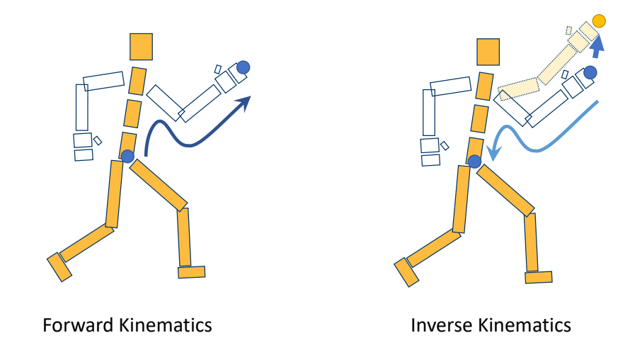
P15
Reference Pose
{ \(𝑅_𝑖 = 𝐼\) }
The pose with zero / identity rotation Bind pose / Reference pose
❗ reference pose不一定是Tpose。
P16
T-Pose? A-Pose?
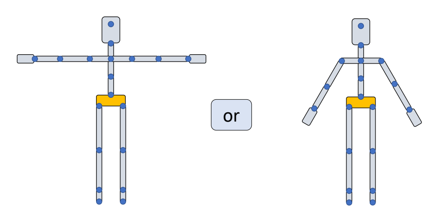

✅ 常见的reference pose一般为Apose或者Tpose。
✅ 对于骨骼动画来讲,\(A\) 或 \(T\) 都一样。
✅ 对于骼骼绑定与蒙皮来讲,更倾向于\(A\)。因为 \(A\) 的肩膀是自然状态。
P19
特殊的reference pose
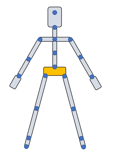 | 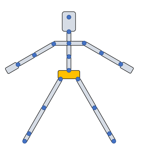 | 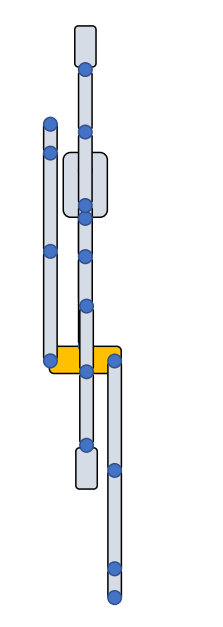 ✅ 这个动作跟建模师建模时的动作镜像操作有关。 |
P23
不同reference pose会引入的问题

✅ 相同的姿态参数放在不同的参考姿态下呈现出的姿态不同。 ✅ 解决方法:Retargeting
P29
Retargeting between reference poses

✅ 让不同参考姿态的角色做出同样的动作,根据 \(R_A\) 求 \(R_B\).
✅ 重定向还有其它问题,例如关节长度、穿模。
P33
Retargeting for a single object
问题分析
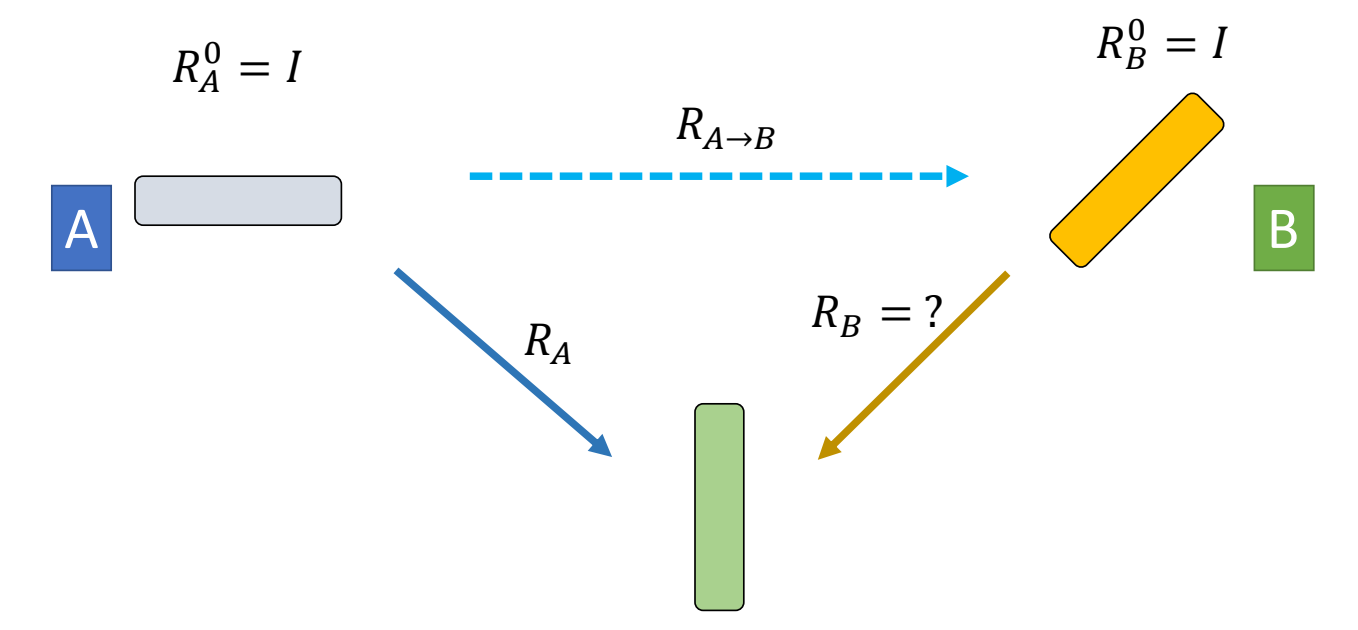
公式推导
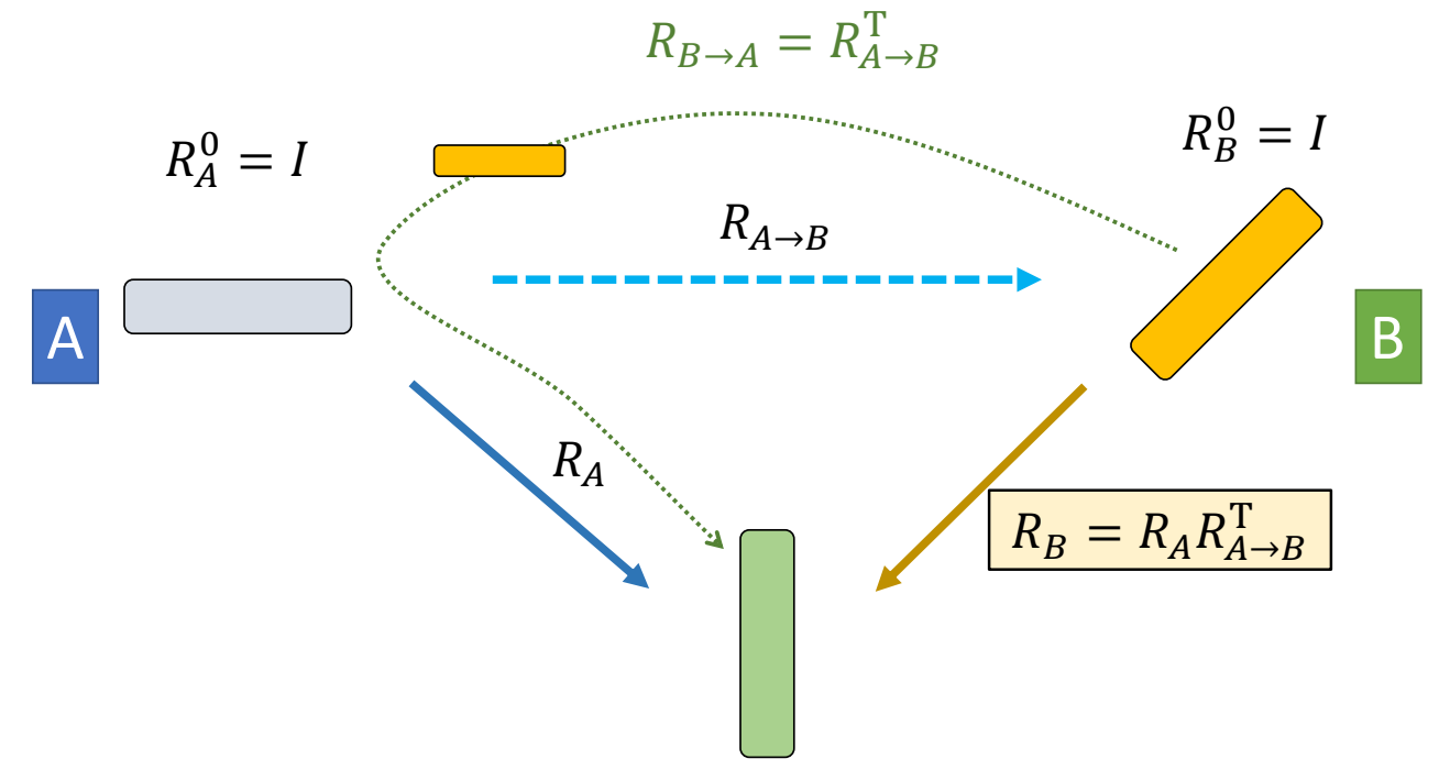
✅ 把 B 先转到 A 的姿态,再做指定动作。
P45
Retargeting for a chain of links
问题分析

✅ 两个关节的场景
公式推导
P49

结论
P51

P52
Retargeting between reference poses
问题分析
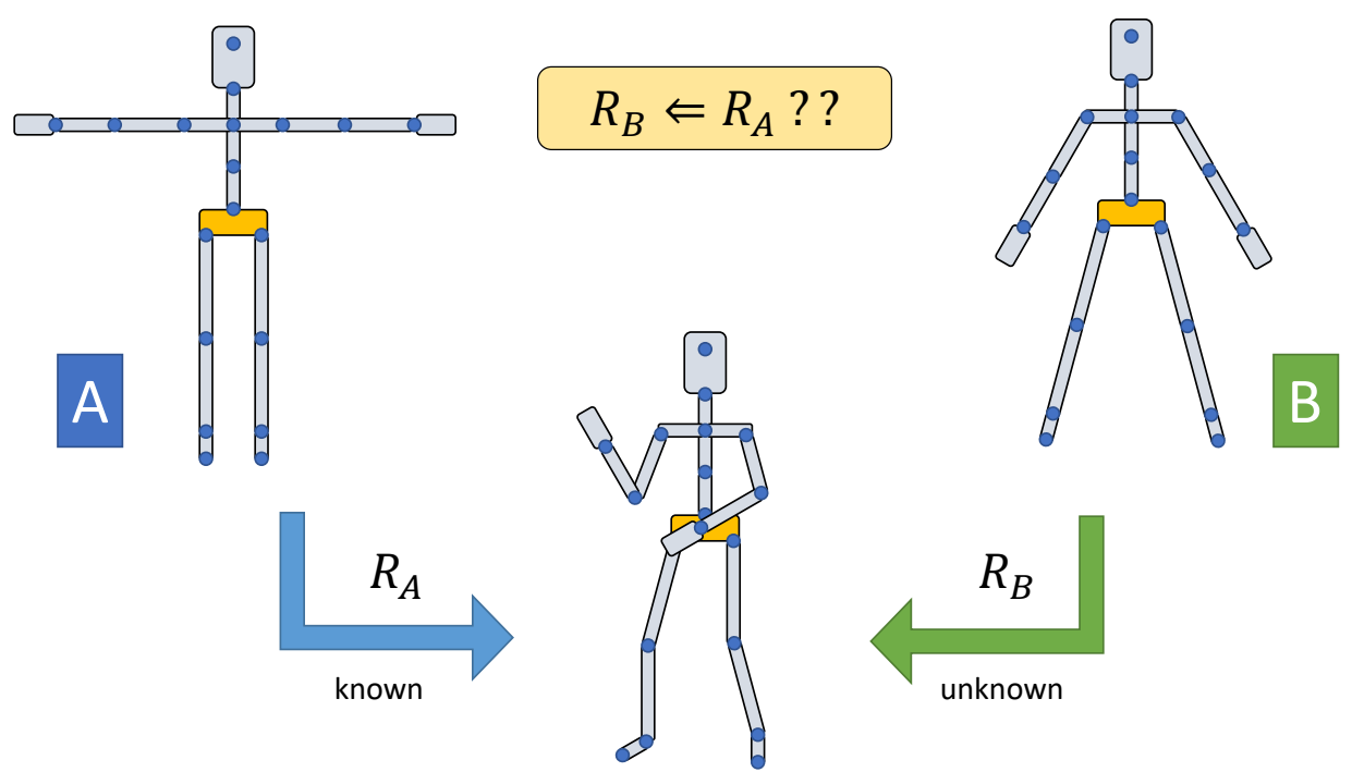
P53
结论

P101
Keyframe Animation and Interpolation
✅ Keyframe Animation跳过
P106
Interpolation
- Given a set of data pairs \(D=\){\((x_i,y_i)\mid i=0,\dots ,N\)} find a function \(f(x)\) such that
P107
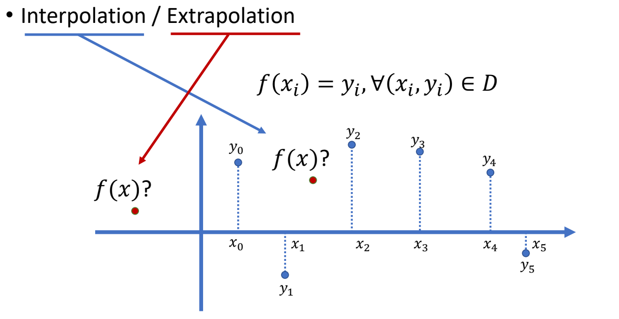
常见的差值方法有Linear Interpolation、Polynomial Interpolation等。详见GAMES102。
P114
Smoothness
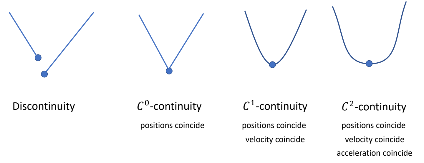
Interpolation of Rotations
P154

P157
SLERP for Quaternions
$$ q_t=\frac{\sin[(1-t)\theta ]}{\sin \theta } q_0 + \frac{\sin t \theta }{\sin \theta }q_1 $$
$$ \cos \theta = q_0 \cdot q_1 $$
Constant rotational speed, but only “linear” interpolation
P158
🔎 Animating rotation with quaternion curves.
Ken Shoemake. 1985
SIGGRAPH Computer Graphics,
本文出自CaterpillarStudyGroup,转载请注明出处。
https://caterpillarstudygroup.github.io/GAMES105_mdbook/
P2
Outline
-
Motion Capture
- History and modern mocap systems
-
Motion Synthesis
- Motion retargeting
- Motion transition
- Motion graph
P3
Motion Capture
How to get motion data?
✅ 动画师制作,光学动捕、视觉动捕,外骨骼动捕,惯性传感器,动作估计。
P29
Motion Synthesis
How to use motion data?
P31
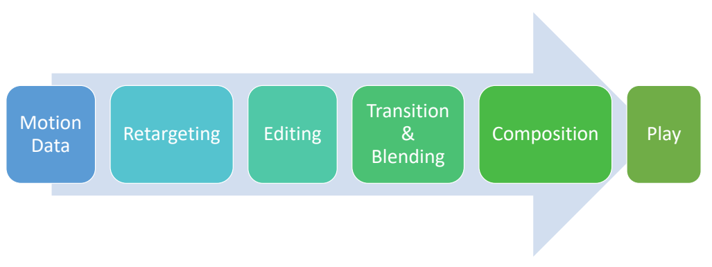
P32
Motion Retargeting
Retargeting要解决的问题
- Retarget a motion to drive a character with
- Different number of bones
- Different bone names
- Different reference pose
- Different bone ratios
- Different skeletal structure
- ……
P34
A possible retargeting pipeline
- Map bone names
- Scale translations
- Copy or retarget joint rotations to fix reference pose
- Postprocessing with IK
- Foot-skating
- Self penetration
- ……
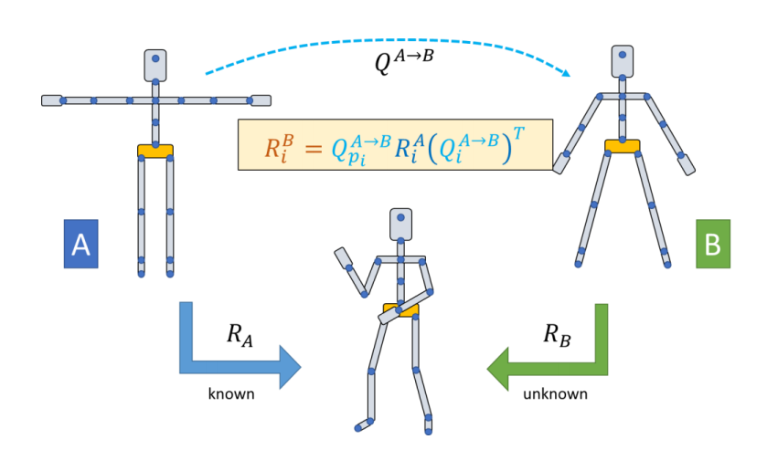
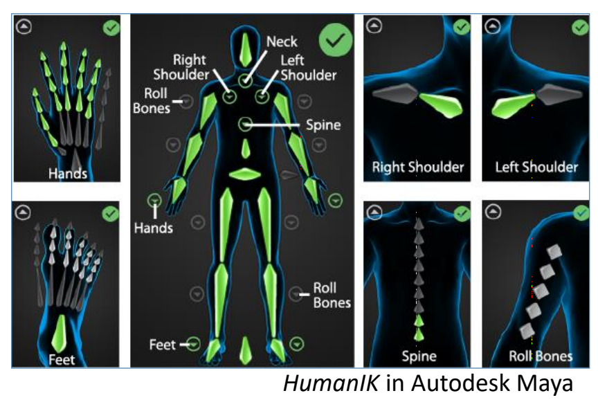
P38
Motion Transition
✅ 有一段走路数据和跑步数据,如何实现人由走到跑的过程。
方法一
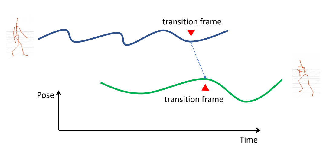 | ✅(1)找到两个 motion 中相似的一帧。 |
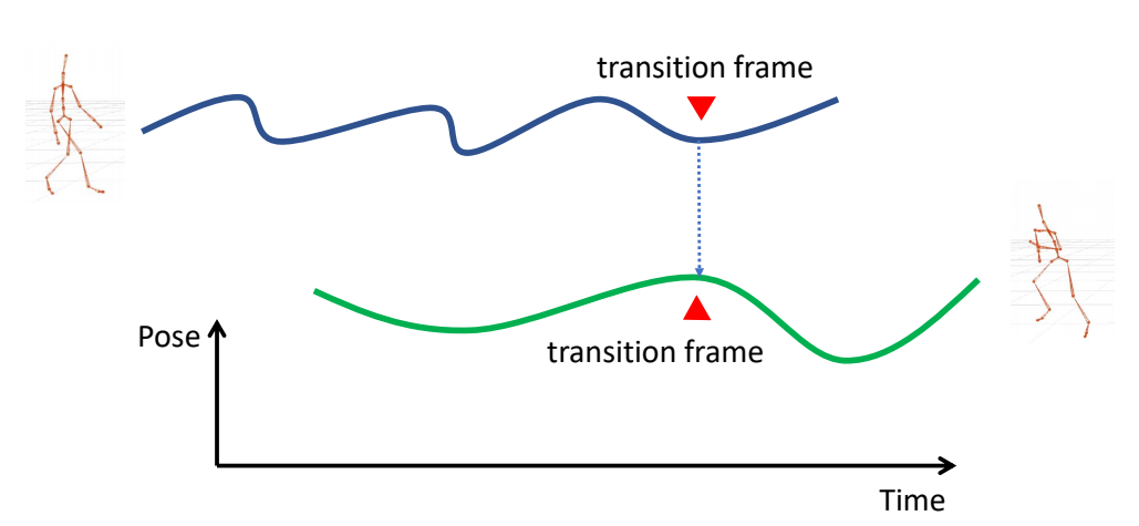 | ✅(2)两帧在时间上对齐 |
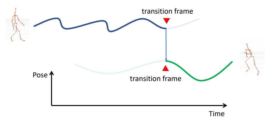 | ✅(3)放到这一帧时动作切换。 |
✅ 缺点:会有明显间断。
方法二
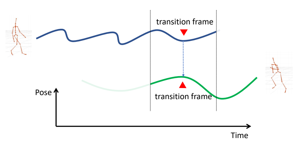 | ✅ 改进:考虑前后帧,并做插值。 |
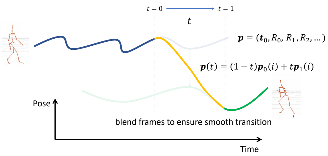 |
P46
$$ p(t)=(1-\phi (t))p_0(i)+\phi (t)p_1(i) $$
✅ 不一定非要线性插值,定义 \(\phi (t)\),或其它混合策略
✅ 可能存在的问题:(1)突然转向(2)滑步
✅ 当走和跑分别是朝不同方法时会出现以上问题。
✅ 解决方法:插值之前动作对齐
P55
“Facing Frame”
定义坐标系
每个角色有自己的角色坐标系,定义为:
A special coordinate system that moves horizontally with the character with one axis pointing to the “facing direction” of the character
✅ 原点:Hip 在地面上的投影
✅ 坐标轴:参考姿态下 \(y\) up \(z\) forward.且旋转和平移都受到限制。
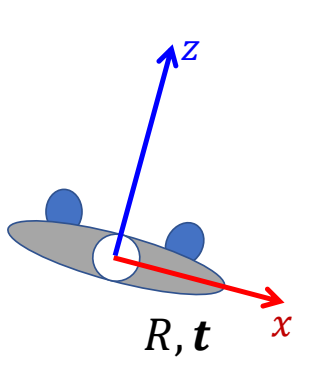
$$ \begin{align*} R & = \theta e_y \\ t & = (t_x,0,t_z) \end{align*} $$
✅ 也可以为不同的的场景定义不同的 \(R\) ,例如上下半身的 \(y\) 轴旋转方向不同。
- Possible definitions of \(R\)
- \(R\) is the y-rotation that aligns the z-axis of the global frame to the heading direction
- \(R\) is the y-rotation that aligns x-axis of the global frame to the average direction of the vectors between shoulders and hips
- Decomposition root rotation as \(R_0=R_yR_{xz}\)
P58
动作分解
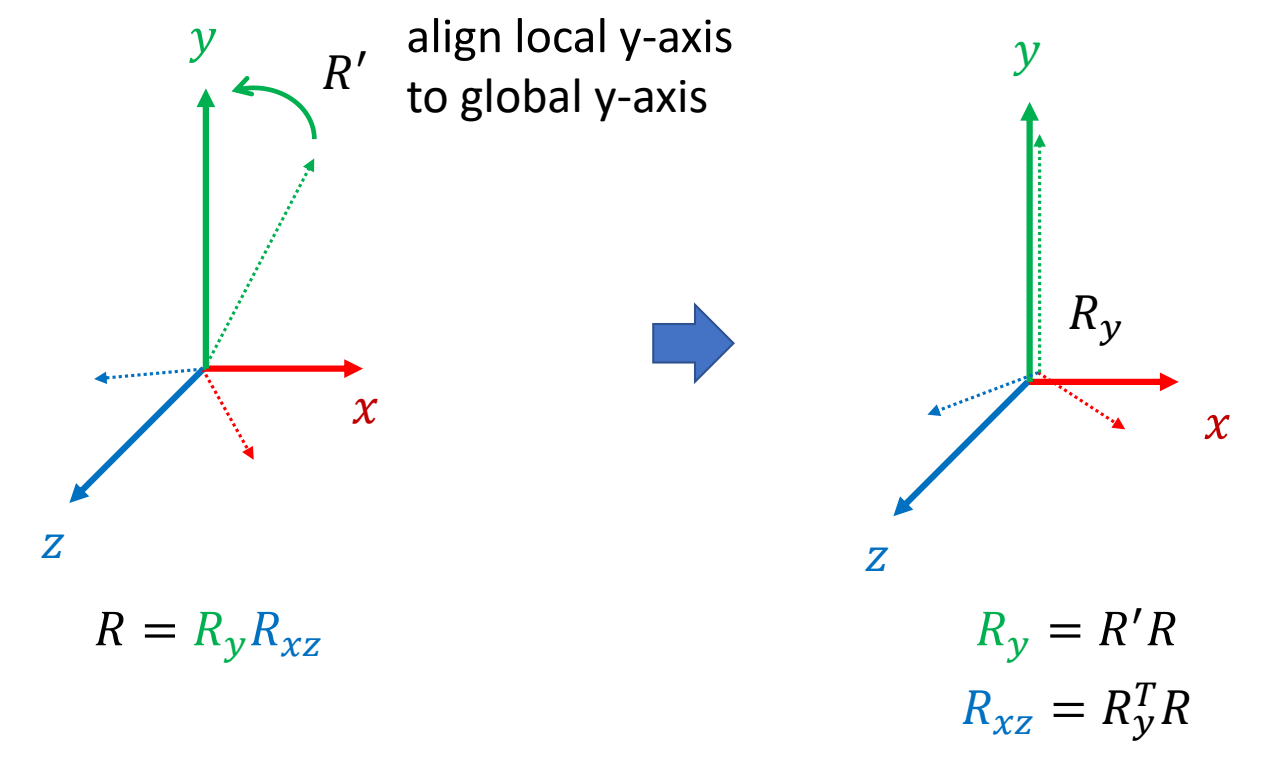
✅ 把 \(R\) 分解为 \(R_y\) 和 \(R_{xz}\),求 \(R_y\)
✅ \({R}' \) 能够把 local y-axis 转到 global y-axis 的矩阵。
P62
动作合成
- How to compute this transformation?
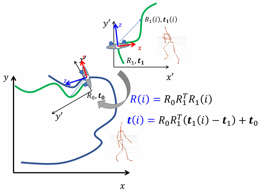
✅ 两个坐标系的转换。
P68
Path Fitting

👆 让角色跟着轨迹移动。
P69
Motion Composition
Computationally generating motions according to
- User control
- Objects in the same environment
- Movements of other characters
- ……
P70
Motion Graphs


👆 动作图的本质是状态机。
P72
Segment Motion Data

✅ 一段动捕数据,如何做分割,如何确定哪些点可以连到一起。
✅ Distance 可以有多种定义方式。
✅ 根据图确定分段与连接。
P73
建立动作转移关系
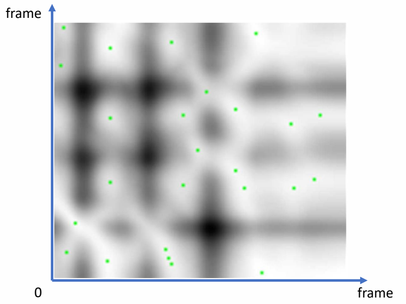
- Distance map
- Each pixel represents the difference between a pair of poses
- Local minima are potential transition point
🔎 Motion graphs Lucas Kovar, Michael Gleicher, and Frédéric Pighin. 2002.
ACM Trans. Graph. 21, 3 (July 2002),
P74
Motion Synthesis
- State-machines
- Nodes represent motion clips
- Edges represent potential transitions
- Transitions are triggered when necessary
- User input
- Clip end
- Check immediate connections for the next clip
- May need deeper search

P75
Interactive Animation Pipeline

✅ 优点:根据路线从动作库中选择最合适的动作,而不是直接使用路线,因此减少滑步。
✅ 缺点:(1) 动作多时动作复杂。
(2) 一个片断播完再切动作,响应较慢。
(3) 需要提前规划好动捕动作。
✅ 如果数据集里没有想要的姿态,可以结合 IK.
P78
Motion Matching?
- Clip → Pose
- Short clip → “Raw” and long motion data
✅ 切换粒度更细:1帧 or 0.1 s.
✅ 灵活性提升,可控性欠缺。
本文出自CaterpillarStudyGroup,转载请注明出处。
https://caterpillarstudygroup.github.io/GAMES105_mdbook/
P1
✅ 基于数据:对现有数据进行连接重组。
✅ 基于学习:对数据处理,放入模型,再生成数据。
P2
Outline
- Recap: interactive character animation
- Motion Graphs
- Motion Matching
- Statistical Models of Human Motion
- Principal Component Analysis
- Gaussian Models
P3
Recap: Interactive Animation
How to make a character respond to user command?
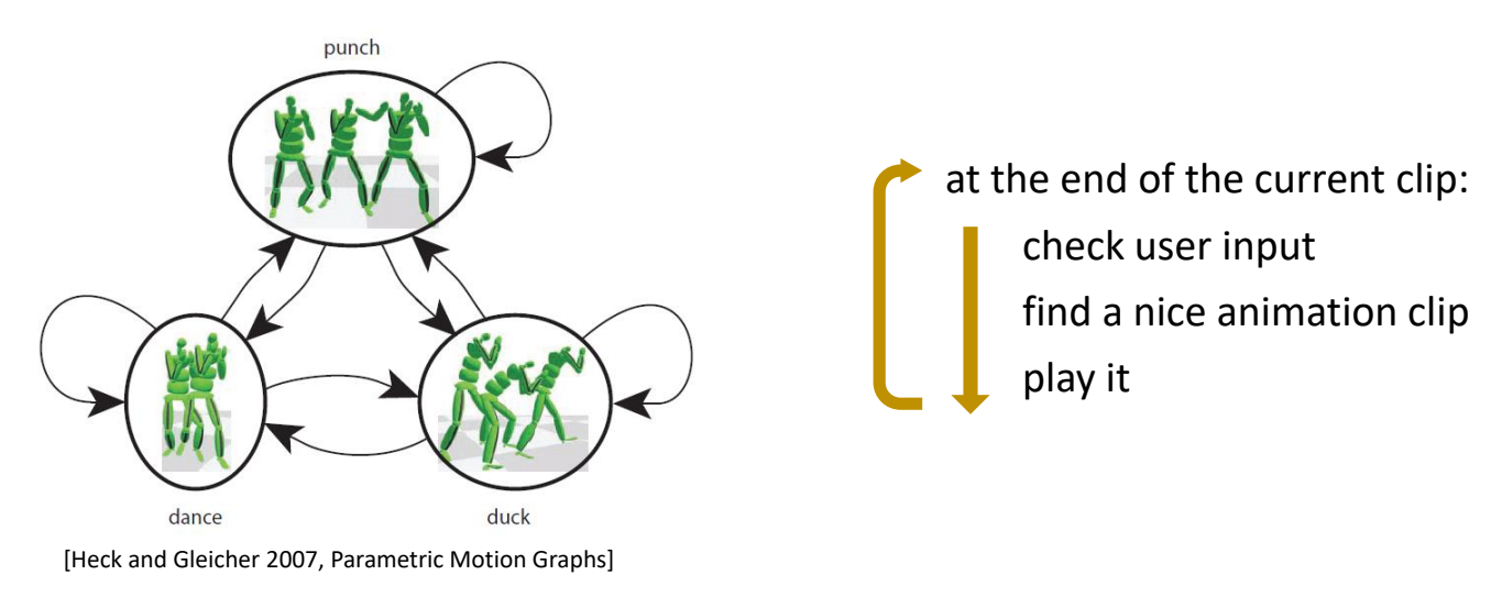
P9
Motion Graphs
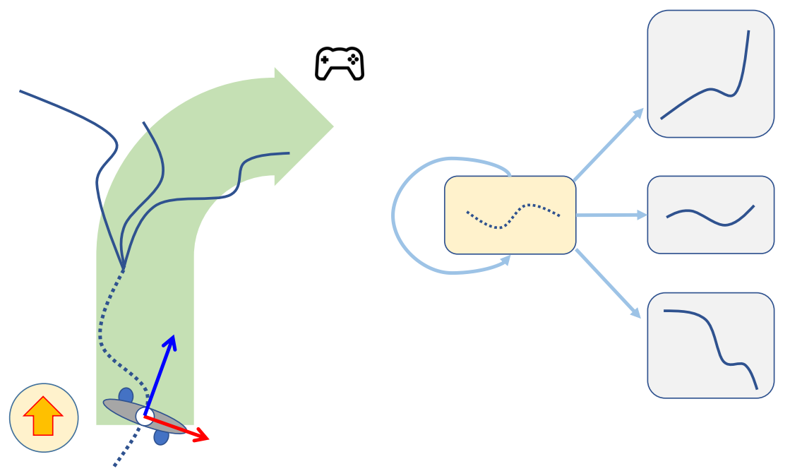
✅ 检测到用户输入后:
- 把当前片段播完(响应慢)
- 所有下一片断与当前状态进行坐标系对齐
- 根据当前状态和预期轨迹,选择下一个片断
- 播放对齐后的下一片断
✅ 可以结合路径规划算,实现一些智能角色。Motion Graph 只是一个底层数据结构。
P14
Motion Fields
| Motion Graphs / State Machines | Motion Fields / Motion Matching |
 | 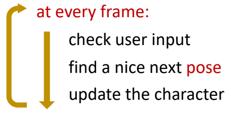 |
✅ Motion Matching 是将 Motion Fields 简化以后加一些比较好的工程实践。
P17
构建 Motion Fields
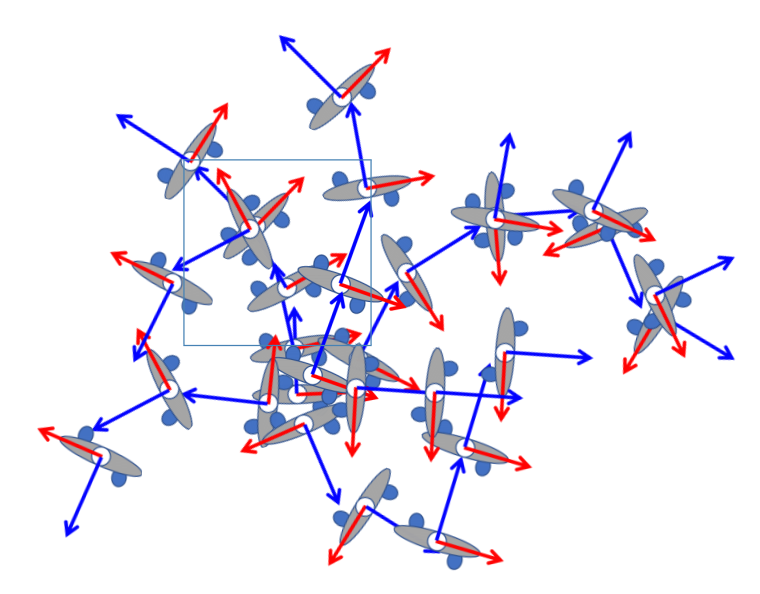
✅ 每条链路代表一个动作,灰圈代表动作里的一帧,整体构成一个很大的 Field.
P20
在Motion Fields中选择pose
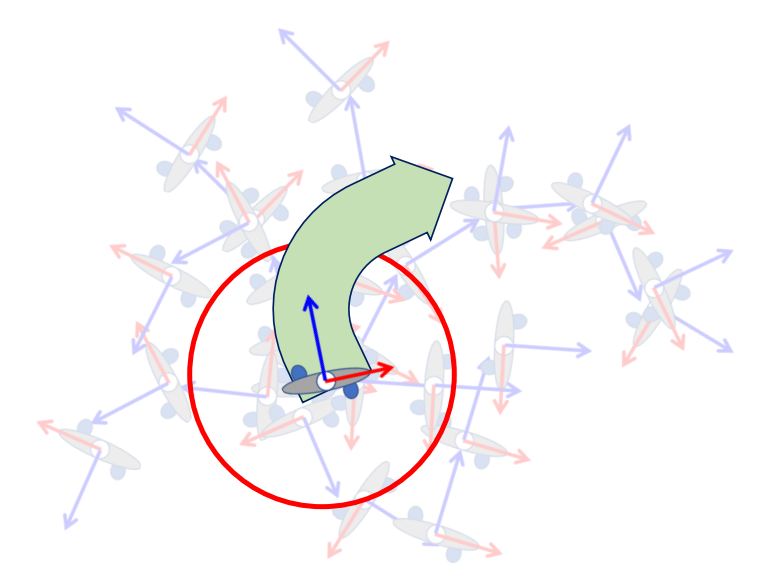
✅ 每一帧有一些最近邻,它们来自不同动作,有不同的状态。
✅ 绿色代表向右,挑出对应帧。做混合。
P23
对pose的混合

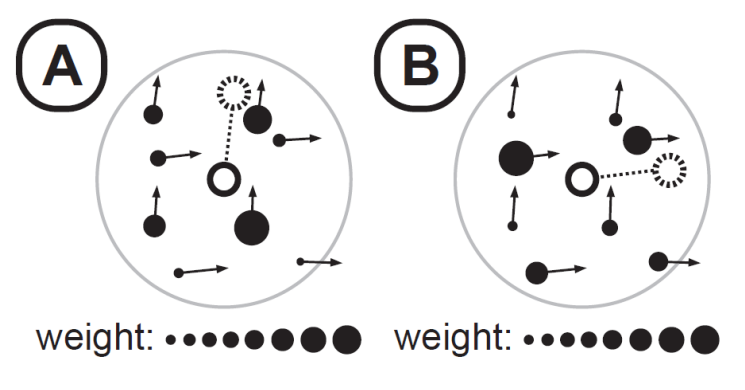
✅ 根据用户输入设置不同权重,会得到不同结果
✅ 优点:(1) 自由控制(2)支持外力,可结果物理仿真(3)不需要使首尾帧相似的预处理。
✅ 缺点:需要设计一些规则来计算最近邻的混合。
✅ 解决方法:强化学习
P24
Pipeline
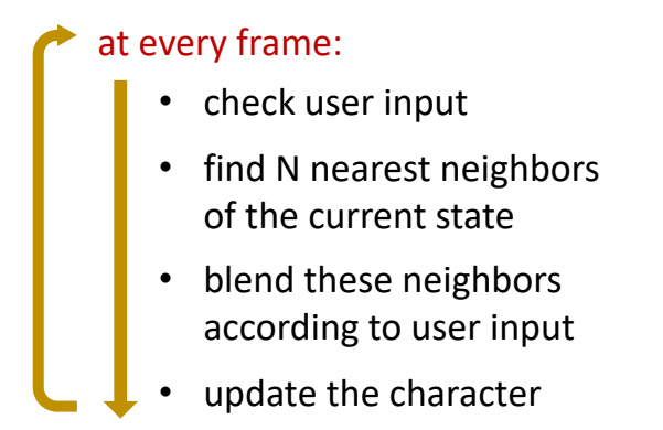
✅ 根据用户输入设计邻局的权重,这一步难以工业化。
✅ 论文使用强化学习来解决,这样增加了训练的难度。
P31
Motion Matching
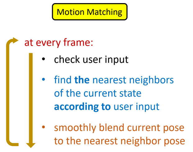
P32
✅ 简化一:只找一个最近邻,不需要 blend. 然后用平滑解决跳变问题。
P34
距离衡量函数
We need a distance function / metric to define the nearest neighbor
$$ \text{next-pose } = \min_{i \in\text{ Dataset}} ||x_{\text{curr}}-x_i|| $$
$$ x: \text{feature vector} $$
✅ Motion Matching 中距离函数的设计很重要,很大程度上影响算法的效果。
✅ 这个距离定义可以是特征相关的。
A possible set of feature vectors:
- root linear/angular velocity
- position of end effectors w.r.t. root joint
- linear/angular velocity of end effectors w.r.t. root joint
- future heading position/orientation (e.g. in 0.5s, 1.0s, 1.5s, etc.)
- foot contacts
- ……
P36
动作平滑
We need a smooth motion
- Only do the search every few frames
- Smoothly blend current pose to the target pose
- Inertialized blending (ref. https://www.theorangeduck.com/page/spring-roll-call by Daniel Holden)
搜索效率
We need a good performance
- An efficient data structure for searching,例如 e.g. KD-tree
数据集
A efficient dataset,例如“Dance card”

✅ 保证所使用的动作集能够覆盖到目标。
✅ 优点:(1) 实现简单 (2) 控制灵活 (3) 可结合物理仿真。
✅ 缺点:(1) 不能解决滑步
P39
Statistical Models of Human Motion
✅ 根据已有数据,对“动作自然”建模。
✅ 或找到一个模型,告诉我们什么是自然姿态。
P43
因为由于以下原因, “自然的动作”实际上是够成高维的动作参数空间的流形曲面。
- Coordinated arm/leg movement
- Musculoskeletal structure
- Laws of physics
- ……
P45
Principal Component Analysis (PCA)
- A technique for
- finding out the correlations among dimensions
- dimensionality reduction
✅ PCA 细节跳过。目的:降维,抓住主要特征。
P65
a pose \(x\) with smaller \(\sum _k\frac{((x-\bar{x})\cdot u_k)^2 }{\sigma ^2_k}\) is more likely to be a good pose

✅ 可作为动作生成的先验,告诉我一个动作是否合理。
✅ \(M_k\) 和 \(\sigma_k\) 分别是 \(k\) 维上的均值和方差。
P66
Character IK with a Motion Prior
正则化先验
$$ F(\theta )=\frac{1}{2} \sum_{i}^{} ||f_i(\theta )-\tilde{x} _i||^2_2+\frac{\lambda }{2}||\theta ||^2_2 $$
$$ \theta=(t_0,R_0,R_1,R_2\dots \dots ) $$
✅ 正则项代表主观先验: \(\theta \) 小更有可能是合理动作。
P68
PCA先验
$$ F(\theta )=\frac{1}{2} \sum_{i}^{} ||f_i(\theta )-\tilde{x} _i||^2_2 $$
$$ +\frac{w }{2}\sum_{k}^{}(\frac{(\theta -\bar{\theta })\cdot u_k }{\sigma _k} )^2 $$
✅ 把 P65 方法应用到 IK 来判断动作好坏的实例。
✅ 改进为基于统计的先验。
P71
Data Distribution
\(p(x)\) : probability that \(x\) is a natural pose
✅ 假设存在这样一个分布,但不知道分布的具体形式,要估计这样的分布
✅(1)从分布中采样,例如:动捕
✅(2)通过各种模型把分布估计出来,即从数据中估计出模型参数。
P75
Gaussian Distribution
✅ 假设分布就是高斯分布
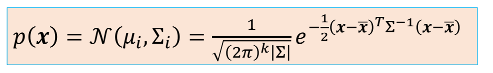
通过Maximum Likelihood Estimators (MLE,最大似然估计)得到:
$$ \begin{align*} \bar{x} &= \frac{1}{N} \sum_{i}^{} x_i \\ \Sigma & =\frac{1}{N} X^TX \end{align*} $$
P76
PCA 可以看作一种高斯分布。
$$ \sum =X^TX=U\begin{bmatrix} \sigma ^2_1 & & & \\ & \sigma ^2_2 & & \\ & & \ddots & \\ & & &\sigma ^2_N \end{bmatrix}U^T $$
$$ x-\bar{x} =\sum_{k=1}^{n} w_ku_k $$
✅ PCA 分解可以看作是坐标转换或变量代换。
P77
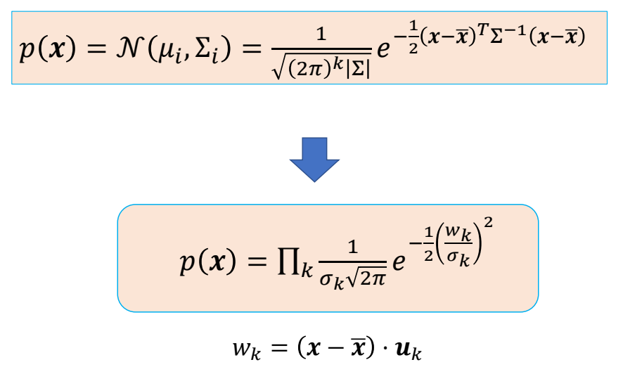
P78
Character IK with a Motion Prior
$$ F(\theta )=\frac{1}{2} \sum_{i} ||f_i(\theta )-\tilde{x} _i||^2_2+\frac{w}{2}\sum_k(\frac{(\theta -\bar{\theta })\cdot u_k }{\sigma _k} )^2 $$
P79
$$ F(\theta )=\frac{1}{2} \sum_{i}^{} ||f_i(\theta )-\tilde{x} _i||^2_2-w \log \prod_k e^{-\frac{1}{2}(\frac{(\theta -\bar{\theta })\cdot u_k }{\sigma _k} )^2 } $$
P80
$$
F(\theta )=\frac{1}{2} \sum_{i}^{} ||f_i(\theta )-\tilde{x} _i||^2_2-w \log p(\theta )
$$
$$ \theta=(t_0,R_0,R_1,R_2\dots \dots ) $$
✅ 第一项:符合目标。第二项:动作合理。
P81
Motion Synthesis with a Motion Prior
Given a motion prior \(p(x)\) learned from a set of data points \(D \)= {\(x_i\)}, Synthesize a motion \(x\) that minimize the objective
$$ f(x)=f(x)-w \log p(x ) $$
Note: \(x\) can represent a pose \(\theta\)
\(\quad\quad\) or a motion clip → a sequence of poses {\( \theta t\)}
\(\quad\quad\) or any features of a motion → e.g. \(w_k\) in PCA
✅ \(x\) 可以不局限于 \(\theta \)、而是任何一个可以描述 motion 的量。
✅ \(f(x)\) 代表目标,目标也不局限于 IK,也可以是Keyframes、User control、Environment constraints等
✅ 但“认为动作符合高斯分布”仍然是一个非常受限约束,难以用于复杂的动作
P83
相关工作
见https://caterpillarstudygroup.github.io/ImportantArticles/index.html
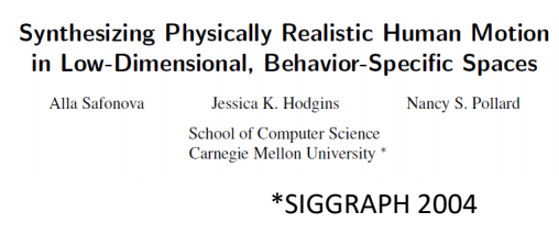 | |
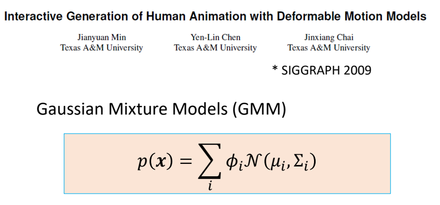 | ✅ 使用高斯混合模型,用于动作编辑。 ✅ \(x\) 不局限于单帧动作,也可以是一个序列。 |
| Min et al. 2009 | ✅ 视频动捕是欠约束问题,但可以通过分布过滤掉不合理的结果。 |
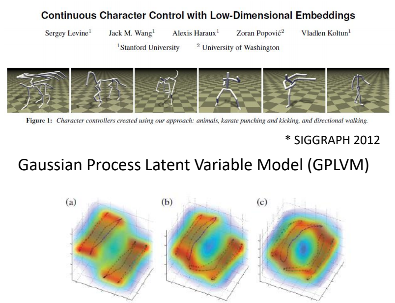 | ✅ 缺点:实现麻烦,很多超参。 |
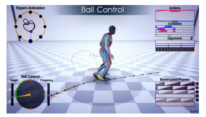 | [Starke et al 2020, Local Motion Phases for Learning Multi-Contact Character Movements] |
 | [Henter et al. 2020, MoGlow: Probabilistic and Controllable Motion Synthesis Using Normalising Flows] ✅ 利用 RL 等方法,在 lalent code 上生成轨迹,再把轨迹转到动作空间。 |
 | [Lee et al 2019, Interactive Character Animation by Learning Multi-Objective Control] |
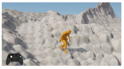 | [Holden et al 2020, Learned Motion Matching] ✅ 用 DL 代替复杂的模型,来估计动作先验。 |
本文出自CaterpillarStudyGroup,转载请注明出处。
https://caterpillarstudygroup.github.io/GAMES105_mdbook/
P2
Outline
- Learning-based Character Animation (cont.)
- Motion Models
- Autoregressive models: PFNN
- Generative models
P4
Learning Motion Models
问题的数学建模
\(p(x)\): probability that 𝒙 is a natural motion
由于 \(p(x)\) 无法由计算得出,所以从数据去学。数据即 a set of example motions {\(x_i\)}∼ \(p(x)\)
P5
数学模型1
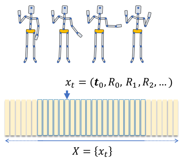
✅ 一个pose可以用每个关节的位置表示,也可以用每个关节的旋转表示。如果用位置约束,最后需要通过IK变成旋转的约束。如果用旋转约束,就难以做到需要约束位置的效果。
✅ P(X)判断整个序列所有pose的联合分布是否合理。
P7
数学模型2
$$ p(X\mid z)=p(x_1,\dots ,x_T\mid z) $$
$$ \begin{align*} 𝑧: & \text{ control parameters} \\ & \text{ latent variables} \\ & …… \end{align*} $$
✅ 对动作序列的要求,除了动作合理,还要符合用户期待,用户要求可以是显式的,例如往左走;也可以是隐式的,例如以老人的风格走。\(z\) 代表用户条件。
✅ P(X|z)判断在条件z下整个序列所有pose的联合分布是否合理。
P8
$$ (x_1,\dots ,x_T)=f(z) $$
$$ \begin{align*} 𝑧: & \text{ control parameters} \\ & \text{ latent variables} \\ & …… \end{align*} $$
✅ 如果概率分布是正确的,基于这个分布采样能得到一个合理的动作,且满足前提条件。
P14
数学模型3
$$ p(X\mid z)=p(x_1,\dots ,x_T\mid z) $$
$$ =p(x_1)\prod_{t}^{} p(x_t\mid x_{t-1},\dots ,x_1;z) $$
\(^\ast \) The chain rule of conditional probabilities:
$$ \begin{align*} p(x_1,x_2,x_3) & = p(x_2,x_3 \mid x_1)p(x_1) \\ & = p(x_3 \mid x_2, x_1)p( x_2 \mid x_1)p(x_1) \end{align*} $$
✅ 序列合理 = 已知序列中的前 \(t-1\) 帧时第 \(t\) 帧应当合理。
P15
采样过程为:
$$ x_t=f(x_{t-1},x_{t-2},\dots x_1;z) $$
P17
数学模型4
✅ 假设动作具有Markov 性(无记忆性)
$$ x_t=f(x_{t-1};z) $$
Markov Property
✅ \(x_t\) 只受 \(x_{t-1}\) 影响,与 \(t-1\) 之前的动作无关。
P18
Two Perspectives on a Motion Sequence
| 数学模型3 | 数学模型4 |
|---|---|
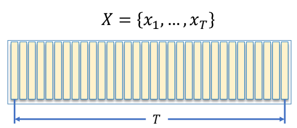 | 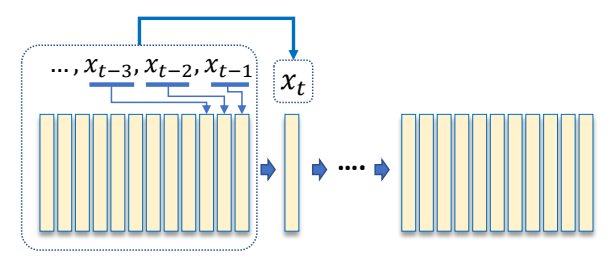 |
 | 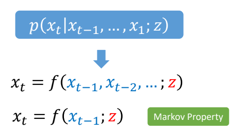 |
| ✅ 无交互无实时通常用前者 | ✅ 游戏里面通常用后者 |
| ✅ 左:直接生成所有动作。 | ✅ 右:一帧一帧地生成。 |
| ✅ 右无法考虑未来,不能根据将要发生的事情调整当前的动作。(自回归) |
P25
数学模型
$$ x_t=f(x_{t-1}) $$

✅ 由于只和上一帧相关,二元组 \((x_{t-1},x_t)\) 构成了一个数据,希望从里面学到一些信息。
✅ Neural Network 相关部分跳过。
✅ 当前先不考虑 \(z\)
✅ 可以把它当作优化问题来解。
P40
Ambiguity Issue
$$ x_t=f(x_{t-1}) $$
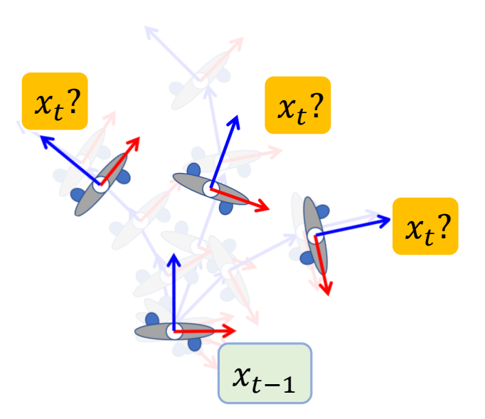
✅ 但是 \(x_t\) 和 \(x_{t-1}\) 的关系是有歧义性的,最后学到一个平均的 \(x_t\).
✅ 因为\(x_{t-1}\)与\(x_t\)不是一对一的mapping关系。
P41
Hidden Variables
$$ x_t=f(x_{t-1};z) $$

✅ 需要加入一个额外的变量,可以来自用户输入或先验信息。关键是怎么找到 \(z\),使学习比较有效。
| ID | Year | Name | Note | Tags | Link |
|---|---|---|---|---|---|
| 113 | 2017 | Phasefunctioned neural networks for character control | PFNN | link |
P55
相关工作
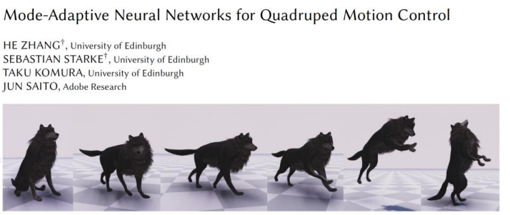 | *SIGGRAPH 2018 ✅ 论文一:除角色姿态,还考虑脚的速度。 |
 | *SIGGRAPH 2020 ✅ 论文二:把两个脚拆开,并考虑手,分别定义相位函数。 |
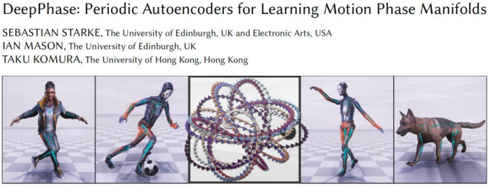 | *SIGGRAPH 2022 ✅ 论文三:从数据中自动学到相位函数的组合。 |
P57
Generative Models
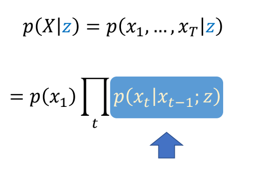
✅ 不学两帧关系,而是直接学概率密度函数。
✅ 难点:(1) 真实 PDF 可能非常复杂 (2) 从一个 PDF 中采样也很难。
✅ PDF 的作用是判断动作是不是真的。
P60
常见套路
| Generative Models | ✅ 一般生成式模型是这样的形式:从一个简单的 PDF,通过 \(f(z)\),映射到 \(p(x)\). ✅ 关键是 \(f(z)\) 要学好。 | 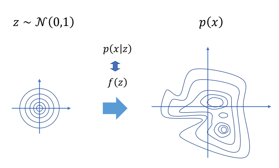 |
| Variational Autoencoders | ✅ VAE:已知一些真实数据采样,用 Encoder 编码到简单分布上的点,再用Decoder 变回原分布上的点。 ✅ control VAE 是 VAE+控制+物理仿真 | 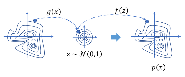 |
| Generative Adversarial Network | ✅ GAN:无 Encoder,增加一个判别器。 ✅ ASE、AMP 是 GAN 的控制版本。 ✅ RL 不结合物理难以 work,因为难以定义 reward. | 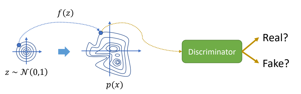 |
| Normalizing Flows | ✅ 标准化流:类似 VAE,使用一个可逆函数。 | 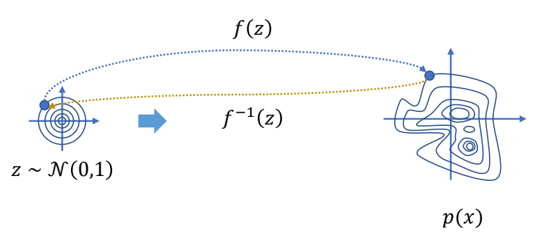 |
| Diffusion Models | ✅ 扩散模型:多次编码与解码。 ✅ 一个动作序列相当于隐空间里的一条轨迹。 | 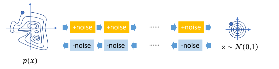 |
P62
相关工作
见https://caterpillarstudygroup.github.io/ImportantArticles/index.html
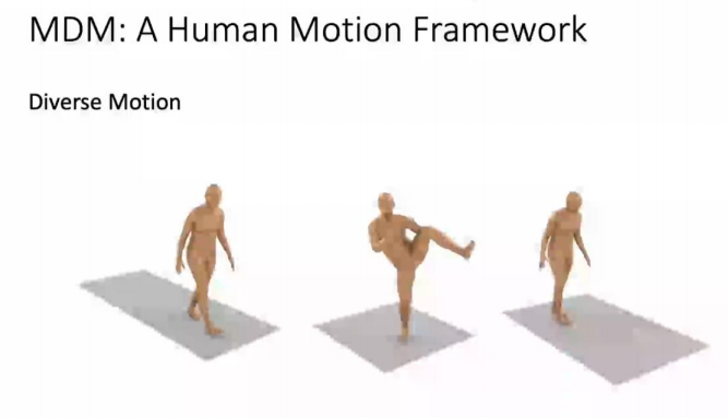 | [Tevet et al. 2022, arXiv, MDM: Human Motion Diffusion Model] |
本文出自CaterpillarStudyGroup,转载请注明出处。
https://caterpillarstudygroup.github.io/GAMES105_mdbook/
基于动力学的角色驱动方法概览
✅ 本章定位:理解如何通过力/力矩驱动角色,生成符合物理规律的动画。
💡 运动学 vs 动力学 的详细对比参见 Introduction
本章知识框架
mindmap
基于动力学的角色驱动
   角色动力学
      仿真
      动力学基础
      关节约束
      接触
   PD 控制
      PD 控制
      PID 控制
      欠驱动问题
   轨迹优化
      优化方法
      数值计算方法
      强化学习方法
   角色控制
      传统方法
      数值方法
      强化学习
✅ 物理方法的难点: ✅ (1) 仿真:在计算机中模拟出真实世界的运行方式。 ✅ (2) 控制:生成角色的动作,来做出响应。 ✅ 角色物理动画通常不关心仿真怎么实现。 ✅ 但也可以把仿真当成白盒,用模型的方法来实现。
动力学方法的四个核心模块
理解动力学方法的四个核心模块:
┌─────────────────────────────────────────────────────────────┐
│  仿真器 (Simulation)                                        │
│  输入:力/力矩 → 输出:新状态                                │
│  核心:Mv̇ + C = f + Jᵀλ                                    │
├─────────────────────────────────────────────────────────────┤
│  底层执行 (PD Control)                                      │
│  输入:目标状态 → 输出:关节力矩 τ                            │
│  核心:τ = k_p(q* - q) + k_d(q̇* - q̇)                       │
├─────────────────────────────────────────────────────────────┤
│  中层策略 (Trajectory/Policy Generation)                    │
│  输入:任务指令 → 输出:目标轨迹/策略                         │
│  ① 轨迹优化:有参考轨迹 (CMA-ES/SAMCON)                     │
│  ② 角色控制:无参考轨迹 (ZMP/IPM/SIMBICON)                  │
│  ③ 强化学习:DeepMimic/AMP/ASE                              │
├─────────────────────────────────────────────────────────────┤
│  高层规划 (Task Planning)                                   │
│  输入:用户意图 → 输出:任务序列                              │
│  方法:有限状态机、行为树                                    │
└─────────────────────────────────────────────────────────────┘
四个模块的关系:
高层规划 → 任务指令
    ↓
中层策略 → 目标轨迹 q*, q̇*  (轨迹优化/角色控制/RL)
    ↓
底层执行 → 关节力矩 τ
    ↓
仿真器 → 新状态
本章子章节:
| 模块 | 文件 | 内容 |
|---|---|---|
| 仿真基础 | Simulation/ | 物理仿真器的工作原理 |
| 约束 | Simulation/JointConstraint.md | 关节约束、接触约束 |
| 执行控制 | PDControl/ | PD 控制原理与应用 |
| 轨迹优化 | Tracking/ | 有参考轨迹的生成方法 |
| 角色控制 | CharacterControl/ | 无参考轨迹的行走控制 |
P4
Physics-based Simulation
✅ 本章定位:理解物理仿真器如何将力/力矩转换为关节旋转。
一、物理仿真概述
1.1 本章要解决的问题
输入:
- 当前状态:位置 \(x\)、旋转 \(R\)、速度 \(v\)、角速度 \(\omega\)
- 外力/力矩:重力、风力、关节力矩(由控制器生成)
- 约束条件:关节约束、接触约束
输出:
- 下一帧状态:新位置 \(x'\)、新旋转 \(R'\)、新速度 \(v'\)、新角速度 \(\omega'\)
核心问题:
给定关节力矩,角色为什么会这样动?
1.2 仿真器与控制器的关系
flowchart LR
    subgraph "控制器"
        C[输入:目标状态/轨迹<br/>输出:关节力矩 τ]
    end

    subgraph "仿真器"
        S[输入:关节力矩 τ<br/>输出:新状态 x', R', v', ω']
    end

    控制器 -- 关节力矩 τ --> 仿真器
    仿真器 -- 新状态<br/>x, R, v, ω --> 控制器
| 模块 | 输入 | 输出 | 核心问题 |
|---|---|---|---|
| 控制器 | 目标状态/轨迹 | 关节力矩 τ | 如何生成力矩让角色达到目标? |
| 仿真器 | 关节力矩 τ | 新状态 | 给定力矩,角色会如何运动? |
分工说明:
- 控制器是「逆向问题」:从目标反推力矩
- 仿真器是「前向问题」:从力矩推算运动
1.3 仿真 Pipeline
根据考虑的约束复杂度,仿真 Pipeline 分为三种:
flowchart TD
    A[当前状态<br/>x, R, v, ω]
    B[计算外力<br/>重力、风力、关节力矩τ]
    C{约束类型?}

    subgraph "Pipeline 1:无约束"
        D1[求解约束力<br/>无约束力]
    end

    subgraph "Pipeline 2:关节约束"
        D2[求解约束力 Jᵀλ<br/>关节约束方程]
    end

    subgraph "Pipeline 3:关节 + 接触"
        D3[接触检测]
        E3[求解约束力<br/>Jᵀλ + 接触力 + 摩擦力]
        D3 --> E3
    end

    A --> B
    B --> C

    C -->|无关节约束 | D1
    C -->|有关节约束 | D2
    C -->|有关节约束 + 接触 | D3

    D1 --> E[积分更新状态<br/>x' = x + v·dt<br/>R', v', ω']
    D2 --> E
    E3 --> E
Pipeline 1:不考虑关节约束
- 每个刚体独立运动
- 适用于自由物体(如抛射物)
- 不适用于角色(角色有关节连接)
Pipeline 2:考虑关节约束
- 关节约束防止刚体分离
- 需求解约束力 \(J^T\lambda\)
- 适用于 Ragdoll、无主动控制的角色
Pipeline 3:考虑关节约束 + 接触摩擦
- 接触约束防止穿透地面
- 摩擦力防止滑动
- 适用于站立、行走的角色
📚 深入学习:
- 运动方程中的力与力矩 - 外力 vs. 关节力矩的详细对比
- 前向动力学与后向动力学 - 运动方程的两种用法
角色的分段刚体表示与仿真
✅ 本章定位:理解如何将角色建模为分段多刚体系统,这是物理仿真的基础。
一、刚体动力学基础
回顾 GAMES103 内容
刚体动力学的核心公式已在 GAMES103 中详细讲解,本节只做简要回顾。
刚体运动方程:
$$ \begin{bmatrix} mI_3 & 0\\ 0 & I \end{bmatrix}\begin{bmatrix} \dot{v} \\ \dot{\omega } \end{bmatrix}+\begin{bmatrix} 0\\ \omega \times I\omega \end{bmatrix}=\begin{bmatrix} f \\ \tau \end{bmatrix} $$
| 符号 | 含义 |
|---|---|
| \(m\) | 质量 |
| \(I\) | 转动惯量张量 |
| \(x, v\) | 位置、线速度 |
| \(R, \omega\) | 旋转、角速度 |
| \(f, \tau\) | 外力、外力矩 |
深入学习:
二、角色的物理仿真表示
从角色模型到仿真模型
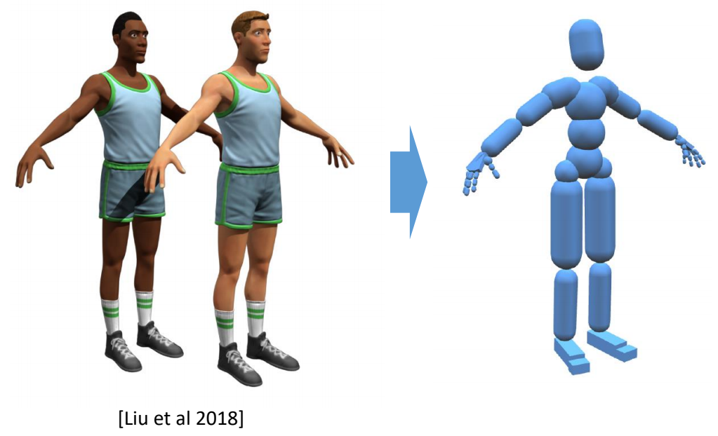
在物理仿真中,角色不能直接使用渲染用的 Mesh,而是需要简化为分段多刚体系统。
仿真角色的组成
Rigid bodies(刚体):
- \(m_i, I_i\) - 质量和转动惯量
- \(x_i, R_i\) - 位置和旋转
- Geometries - 碰撞几何体(仿真中使用简单几何体代替 Mesh)
Joints(关节):
- Position - 关节位置
- Type - 关节类型(Hinge、Universal、Ball 等,决定约束方程)
- Bodies - 连接的刚体
✅ 关节的数量比刚体的数量少 1
碰撞几何体的选择
| 身体部位 | 常用几何体 | 原因 |
|---|---|---|
| 头部 | 球体 | 形状接近、计算简单 |
| 躯干 | 胶囊体/盒体 | 近似 torso 形状 |
| 手臂/腿 | 胶囊体 | 细长形状 |
| 手/脚 | 盒体 | 便于接触检测 |
✅ 使用简单几何体可以大幅提高碰撞检测和约束求解的效率。
在物理引擎中定义角色
在物理引擎中创建一个刚体需要提供:
Masses:     m, I           // 质量和转动惯量
Kinematics: x, v, R, ω    // 运动学状态
Geometry:   Box/Sphere/Capsule/Mesh  // 碰撞几何体
            Collision detection      // 碰撞检测
            Compute m, I             // 计算质量属性
三、分段多刚体动力学
从单刚体到多刚体
单刚体: $$ M\dot{v} + C(x,v) = f $$
其中 \(M\) 和 \(C\) 是分块对角矩阵,每个刚体独立。
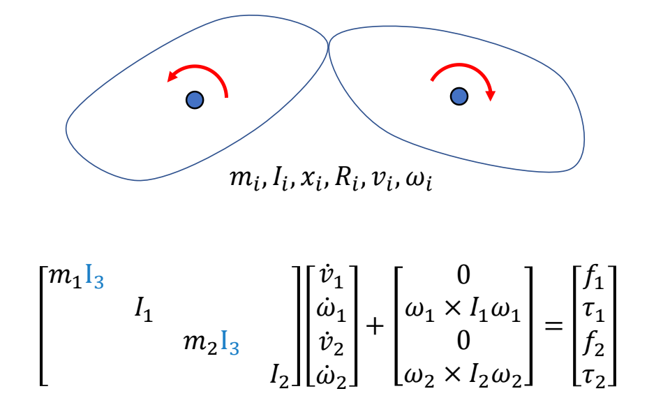
✅ 两个刚体如果独立,可以以矩阵的方式扩展。
✅ 分段多刚体在公式上没有本质区别,只是矩阵更大。
对于 \(n\) 个刚体的系统:
- \(M\) 是 \(6n \times 6n\) 的分块对角矩阵
- \(C(x,v)\) 是 \(6n\) 维向量
多刚体系统的扩展
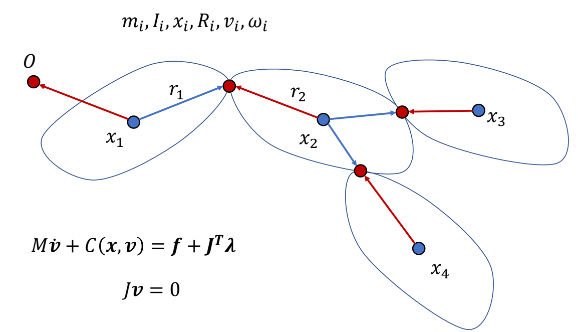
✅ 关于约束力的说明:当刚体通过关节连接时,需要添加约束力 \(J^T\lambda\)。这部分内容在后续章节详细讲解。
与后续章节的关系
| 本节内容 | 后续应用 |
|---|---|
| 刚体动力学基础 | 理解单个身体的运动 |
| 角色仿真表示 | 碰撞检测、接触求解 |
| 分段多刚体公式 | 所有仿真章节的基础 |
约束求解专题(本节不涉及):
- Constraints.md - 约束求解原理(小球例子)
- JointConstraint.md - 关节约束推导
- Contacts.md - 接触模型
- SimulationPipeline.md - 完整仿真流程
小结
角色物理仿真的建模流程:
角色 Mesh → 简化为刚体 → 添加关节 → 定义碰撞几何体 → 分段多刚体系统
核心公式(无约束情况): $$ M\dot{v} + C(x,v) = f $$
| 项 | 含义 |
|---|---|
| \(M\dot{v} + C(x,v)\) | 惯性力(质量 + 科氏力/离心力) |
| \(f\) | 外力(重力、风力、关节力矩) |
✅ 本节只介绍分段多刚体的表示方法。当刚体通过关节连接时,需要添加约束力 \(J^T\lambda\),详见后续章节。
本文出自 CaterpillarStudyGroup,转载请注明出处。 https://caterpillarstudygroup.github.io/GAMES105_mdbook/
Constraints 简化问题分析
💡 为什么先学小球? 接下来要介绍关节约束的求解。在讲解角色的关节约束之前,先用小球的简单例子来理解约束求解的核心思想。 小球约束与关节约束的数学形式完全相同,只是场景更简单、更容易理解。
问题描述
✅ 假设有一约束:小球必须按轨道行进。

小球速度分析
✅ 根据已知条件,可以进行以下分析:由于每一时刻都满足,对时间求导,导数为零。

其中第一项为 \(g(x)\) 的雅克比矩阵,记作 \(J\) 或 \([\nabla g]^{T}\), 第二项为 \(x\) 的速度。 因此得到约束为:如果要求小球按照轨道运行,其速度必须满足以下公式。
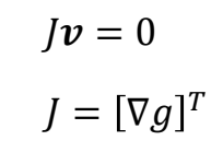
小球的约束力分析
✅ 为了让小球满足约束,需给小球一个约束力。
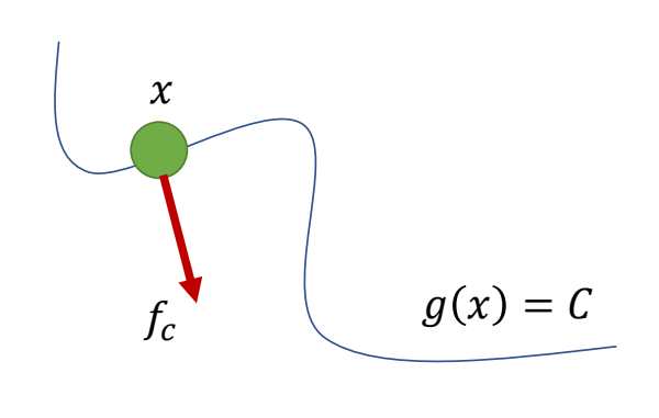
\(^\ast \) Constraint is passive No energy gain or loss!!!
$$ f_c\cdot v=0 $$
✅ 约束力不应产生能量,即力与运动方向垂直。
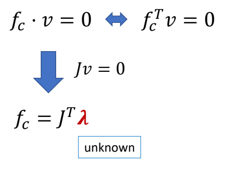
✅ \(J\) 本是一个矩阵,但在这个场景中 \(C\) 是常数,所以 \(J\) 是向量。 ✅ 结合是一页的结论可知:\(f_c\) 与 \(J\) 同方向,但大小未知。\(\lambda \)代表一个未知的 scale。 ✅ \(f_c\) 大小以当前状态和外力情况计算而得。
小球的整体受力分析
✅ 对小球做受力分析,受到外力 \(f\) 和约束力 \(f_c\). ✅ 假设 \(M,x,v.f\) 已知,求 \(f_c\) ,使得小球沿轨迹移动。

$$ \begin{align*} M\dot{v} & =f+J^T\lambda \\ Jv&=0 \end{align*} $$
✅ 公式 1:\(f=am\).公式 2:前面推导得出。把两个公式离散化。 ✅ 假设当前时刻已满足 \(J_n v_n = 0\),所以只约束下一时刻。
$$ \begin{align*} M\frac{v_{n+1}-v_n}{h} & =f+J^T\lambda \\ Jv_{n+1}&=0 \end{align*} $$
✅ 得出未知数为\(\lambda\)和\(v_{n+1}\)的联立方程组,求解方程组。 ✅ 因为公式 2 只约束了速度没有约束位置。离散化后对原公式只是近似,会有误差,导到小球远离曲线。 ✅ 解方程组不难,但存在小球偏离轨道的问题。
✅ 当物体偏离轨道,要把它拉回来。因此公式 2 改为:
$$ Jv_{n+1}=\alpha \frac{C-g(x_n)}{h} $$
等式右边的非零项称为 Correction of numerical errors。 𝛼: error reduction parameter (ERP)
方程组求解
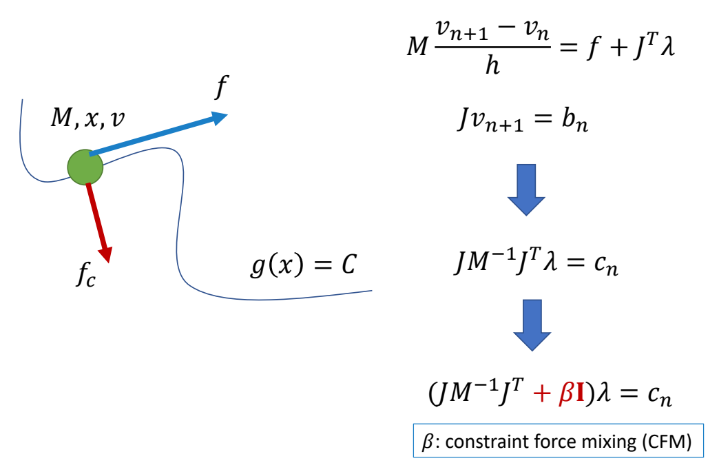
✅ 把校正项简写为 \(b\). \( n \) 时刻发现的误差由 \( n+1 \) 时刻来校正。 ✅ 为了防止矩阵不可逆,增加 \(\beta I\).(常见技巧) ✅ 解 \(\lambda\) 需要先求逆。
附录:公式推导过程
目标:求解拉格朗日乘子 \(\lambda\)
已知方程组(带误差校正):
$$ \begin{cases} \displaystyle M\frac{v_{n+1}-v_n}{h} = f + J^T\lambda \\ Jv_{n+1} = b \end{cases} $$
其中 \(b = \alpha\frac{C-g(x_n)}{h}\) 是误差校正项。
步骤 1:从运动方程解出 \(v_{n+1}\)
$$ M\frac{v_{n+1}-v_n}{h} = f + J^T\lambda $$
$$ v_{n+1}-v_n = h M^{-1}(f + J^T\lambda) $$
$$ v_{n+1} = v_n + h M^{-1}f + h M^{-1}J^T\lambda $$
令 \(v^* = v_n + h M^{-1}f\)(不含约束力的预测速度)
则: $$ v_{n+1} = v^* + h M^{-1}J^T\lambda $$
步骤 2:代入约束方程
约束方程: $$ Jv_{n+1} = b $$
代入 \(v_{n+1}\): $$ J(v^* + h M^{-1}J^T\lambda) = b $$
展开: $$ Jv^* + h J M^{-1}J^T\lambda = b $$
步骤 3:解出 \(\lambda\)
$$ h J M^{-1}J^T\lambda = b - Jv^* $$
$$ \lambda = (h J M^{-1}J^T)^{-1}(b - Jv^*) $$
步骤 4:防止矩阵不可逆
\(J M^{-1}J^T\) 可能不可逆(例如约束冗余时),添加正则化项 \(\beta I\):
$$ \lambda = (J M^{-1}J^T + \beta I)^{-1}(b - Jv^*) $$
最终公式
$$ \boxed{\lambda = (J M^{-1}J^T + \beta I)^{-1}(b - Jv^*)} $$
| 符号 | 含义 |
|---|---|
| \(v^* = v_n + h M^{-1}f\) | 无约束时的预测速度 |
| \(b = \alpha\frac{C-g(x_n)}{h}\) | 误差校正项(ERP) |
| \(\beta I\) | 防止矩阵不可逆的正则化项 |
✅ 核心思想:把约束求解转化为求解拉格朗日乘子 \(\lambda\) 的线性方程组。
从小球到关节约束
小球例子的约束求解公式可以直接应用到关节约束。
| 概念 | 小球例子 | 关节约束 |
|---|---|---|
| 约束对象 | 小球位置 | 两个刚体的连接点 |
| 约束方程 | \(g(x) = 0\)(小球在轨道上) | \(x_1 + R_1r_1 = x_2 + R_2r_2\)(连接点重合) |
| 速度级约束 | \(Jv = 0\) | \(v_1 + \omega_1 \times r_1 = v_2 + \omega_2 \times r_2\) |
| 雅克比 J | 向量(\(1 \times 6\)) | 矩阵(\(3 \times 12\)) |
| 约束力 | \(J^T\lambda\)(轨道支持力) | \(J^T\lambda\)(关节力) |
| 物理意义 | 防止小球脱离轨道 | 防止刚体分离 |
关节约束的约束方程推导
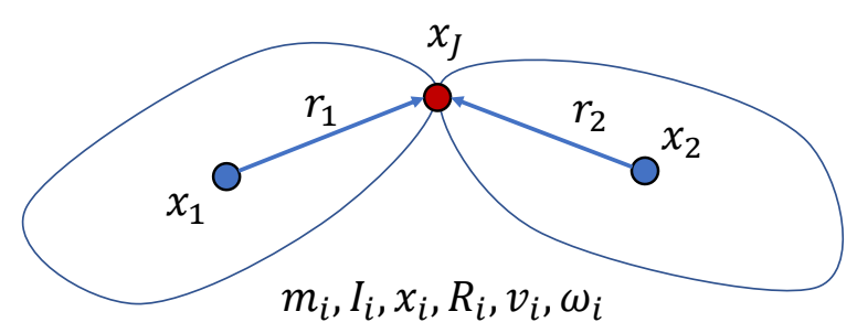
✅ 关节约束:两个刚体在关节处的位置必须相同。
位置级约束: $$ x_1 + R_1 r_1 = x_2 + R_2 r_2 $$
速度级约束(对时间求导): $$ v_1 + \omega_1 \times r_1 = v_2 + \omega_2 \times r_2 $$
矩阵形式: $$ \begin{bmatrix} I_3 & -[r_1]\times & -I_3 & [r_2]\times \end{bmatrix} \begin{bmatrix} v_1 \\ \omega_1 \\ v_2 \\ \omega_2 \end{bmatrix} = 0 $$
简化为: $$ Jv = 0 $$
✅ 数学形式完全相同:\(M\dot{v} + C = f + J^T\lambda\),\(Jv = b\) 只是 \(J\) 的具体形式不同(小球是向量,关节是矩阵)。
深入学习:JointConstraint.md - 关节约束详细推导(各种关节的 \(J\) 矩阵构造与统一求解框架)
关节约束
💡 前置知识:关于角色的分段刚体表示,见 RigidBodyRepresentation.md
关节类型与约束方程
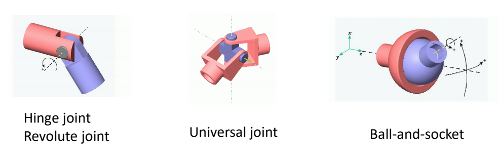
| 关节类型 | 约束自由度 | 位置约束 | 角速度约束 |
|---|---|---|---|
| Ball Joint(球铰) | 3 个平移 | ✅ | ❌ |
| Hinge Joint(铰链) | 3 个平移 + 2 个旋转 | ✅ | ✅ |
| Universal Joint(万向节) | 3 个平移 + 1 个旋转 | ✅ | ✅ |
| Fixed Joint(固定) | 3 个平移 + 3 个旋转 | ✅ | ✅ |
Ball Joint(球铰)
✅ Ball Joint 只约束位置,允许三个方向的自由旋转。
约束方程
位置级约束: $$ x_1 + R_1 r_1 = x_2 + R_2 r_2 $$
速度级约束(对时间求导): $$ v_1 + \omega_1 \times r_1 = v_2 + \omega_2 \times r_2 $$
矩阵形式: $$ J = \begin{bmatrix} I_3 & -[r_1]\times & -I_3 & [r_2]\times \end{bmatrix} $$
$$ \begin{bmatrix} I_3 & -[r_1]\times & -I_3 & [r_2]\times \end{bmatrix} \begin{bmatrix} v_1 \\ \omega_1 \\ v_2 \\ \omega_2 \end{bmatrix} = 0 $$
简化为: $$ Jv = 0 $$
其中 \(J\) 是 \(3 \times 12\) 矩阵。
Hinge Joint(铰链)
✅ Hinge Joint 约束位置 + 2 个旋转自由度,只允许绕铰链轴旋转。
约束方程
位置级约束(同 Ball Joint): $$ x_1 + R_1 r_1 = x_2 + R_2 r_2 $$
角速度约束(额外约束): $$ \omega_1 \cdot a_1 = \omega_2 \cdot a_2 $$
其中 \(a_1, a_2\) 是两个刚体上的铰链轴方向向量。
矩阵形式: $$ Jv = \begin{bmatrix} J_{\text{pos}} \\ J_{\text{ang}} \end{bmatrix} v = 0 $$
其中:
- \(J_{\text{pos}}\) 是 \(3 \times 12\) 的位置约束矩阵(同 Ball Joint): $$ J_{\text{pos}} = \begin{bmatrix} I_3 & -[r_1]\times & -I_3 & [r_2]\times \end{bmatrix} $$
- \(J_{\text{ang}}\) 是 \(2 \times 12\) 的角速度约束矩阵,约束两个刚体在垂直于铰链轴方向上的角速度分量相等: $$ J_{\text{ang}} = \begin{bmatrix} 0_3 & a_{1\perp 1}^T & 0_3 & -a_{2\perp 1}^T \\ 0_3 & a_{1\perp 2}^T & 0_3 & -a_{2\perp 2}^T \end{bmatrix} $$ 其中 \(a_{\perp 1}, a_{\perp 2}\) 是两个垂直于铰链轴的方向。
完整 $J$ 矩阵是 \(5 \times 12\): $$ J = \begin{bmatrix} I_3 & -[r_1]\times & -I_3 & [r_2]\times \\ 0_3 & a_{1\perp 1}^T & 0_3 & -a_{2\perp 1}^T \\ 0_3 & a_{1\perp 2}^T & 0_3 & -a_{2\perp 2}^T \end{bmatrix} $$
Universal Joint(万向节)
✅ Universal Joint 约束位置 + 1 个旋转自由度,允许两个旋转自由度。
约束方程
位置级约束(同 Ball Joint): $$ x_1 + R_1 r_1 = x_2 + R_2 r_2 $$
角速度约束(额外约束): $$ \omega_1 \cdot a_1 = \omega_2 \cdot a_2 $$ $$ \omega_1 \cdot b_1 = \omega_2 \cdot b_2 $$
其中 \(a, b\) 是两个相互垂直的轴向,分别位于两个刚体上。
矩阵形式: $$ Jv = \begin{bmatrix} J_{\text{pos}} \\ J_{\text{ang}} \end{bmatrix} v = 0 $$
其中:
- \(J_{\text{pos}}\) 是 \(3 \times 12\) 的位置约束矩阵(同 Ball Joint)
- \(J_{\text{ang}}\) 是 \(1 \times 12\) 的角速度约束矩阵,约束两个刚体在万向节轴向上的角速度分量相等: $$ J_{\text{ang}} = \begin{bmatrix} 0_3 & a_1^T & 0_3 & -a_2^T \end{bmatrix} $$
完整 $J$ 矩阵是 \(4 \times 12\): $$ J = \begin{bmatrix} I_3 & -[r_1]\times & -I_3 & [r_2]\times \\ 0_3 & a_1^T & 0_3 & -a_2^T \end{bmatrix} $$
Fixed Joint(固定)
✅ Fixed Joint 完全固定两个刚体,不允许任何相对运动。
约束方程
位置级约束(同 Ball Joint): $$ x_1 + R_1 r_1 = x_2 + R_2 r_2 $$
角速度约束(全部约束): $$ \omega_1 = \omega_2 $$
矩阵形式: $$ Jv = \begin{bmatrix} J_{\text{pos}} \\ J_{\text{ang}} \end{bmatrix} v = 0 $$
其中:
- \(J_{\text{pos}}\) 是 \(3 \times 12\) 的位置约束矩阵(同 Ball Joint)
- \(J_{\text{ang}}\) 是 \(3 \times 12\) 的角速度约束矩阵,约束两个刚体的角速度完全相同: $$ J_{\text{ang}} = \begin{bmatrix} 0_3 & I_3 & 0_3 & -I_3 \end{bmatrix} $$
完整 $J$ 矩阵是 \(6 \times 12\): $$ J = \begin{bmatrix} I_3 & -[r_1]\times & -I_3 & [r_2]\times \\ 0_3 & I_3 & 0_3 & -I_3 \end{bmatrix} $$
运动方程 + 约束方程
无论哪种关节,都可以统一写成:
$$ \begin{align*} M\dot{v} + C(x,v) &= f + J^T\lambda \\ Jv &= 0 \end{align*} $$
| 符号 | 含义 |
|---|---|
| \(M\) | \(6n \times 6n\) 质量矩阵 |
| \(C(x,v)\) | 科氏力 + 离心力 |
| \(f\) | 外力(重力、风力、关节力矩) |
| \(J\) | 约束雅克比矩阵(\(m \times 6n\)) |
| \(\lambda\) | 拉格朗日乘子(约束力大小) |
✅ 联立方程组可以解出约束力 \(\lambda\) 和下一时刻的速度。
约束求解的详细推导:见 Constraints.md(小球例子)
统一约束求解框架
✅ 核心洞察:不同约束的求解公式完全一样,唯一的区别是雅克比矩阵 \(J\) 的构造。
不同关节的 \(J\) 矩阵对比
| 关节类型 | \(J\) 的行数 | 说明 |
|---|---|---|
| Ball Joint | 3 行 | 仅位置约束 |
| Hinge Joint | 5 行 | 3 行位置约束 + 2 行角速度约束 |
| Universal Joint | 4 行 | 3 行位置约束 + 1 行角速度约束 |
| Fixed Joint | 6 行 | 3 行位置约束 + 3 行角速度约束 |
统一求解流程
无论哪种关节,都遵循相同的求解步骤:
- 计算预测速度:\(v^* = v_n + h M^{-1}f\)
- 构建约束雅可比 \(J\)(根据关节类型)
- 求解拉格朗日乘子: $$ \lambda = (J M^{-1}J^T + \beta I)^{-1}(b - Jv^*) $$
- 计算约束力:\(f_c = J^T\lambda\)
- 更新速度:\(v_{n+1} = v^* + h M^{-1}J^T\lambda\)
✅ 物理引擎实现的关键:
- 为每种关节类型实现一个 \(J\) 矩阵构造函数
- 把所有约束的 \(J\) 行堆叠起来形成总约束矩阵
- 代入统一公式求解 \(\lambda\)
✅ 多约束同时处理:当系统有多个约束时(如多个关节 + 接触),只需将每个约束的 \(J\) 矩阵按行堆叠,公式形式不变,只是矩阵维度更大。
多个刚体与多个约束
✅ 分段多刚体系统:公式形式相同,只是矩阵维度更大。
对于 \(n\) 个刚体、\(m\) 个约束的系统:
- \(M\) 是 \(6n \times 6n\) 的分块对角矩阵
- \(J\) 是 \(m \times 6n\) 的矩阵(每个约束贡献若干行)
关节力矩
关节力矩的详细介绍:见 JointTorques.md
✅ 关节力矩是主动控制力矩,用于驱动角色运动。在运动方程中: $$ M\dot{v} + C(x,v) = f_{\text{ext}} + f_{\text{joint}} + J^T\lambda $$ 其中 \(f_{\text{joint}}\) 是关节力矩(主动),\(J^T\lambda\) 是约束力(被动)。
本文出自 CaterpillarStudyGroup,转载请注明出处。 https://caterpillarstudygroup.github.io/GAMES105_mdbook/
关节力矩(Joint Torques)
🛈 前置知识:关于关节约束的数学形式,见 JointConstraint.md
:::info 核心要点
- 关节力矩是主动控制输入,用于驱动角色运动
- 施加方式:在一个刚体上加 $\tau$,另一个加 $-\tau$
- 与外力不同:关节力矩只产生旋转,不产生平移
:::
什么是关节力矩
关节力矩(Joint Torques) 是角色控制中的核心概念。它是在关节上施加的主动控制力矩,用于驱动角色运动。
物理意义
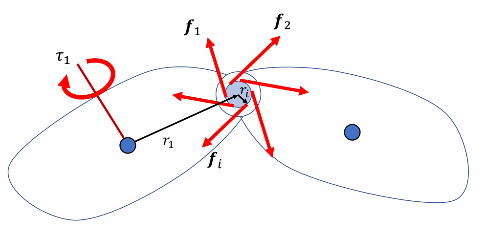
✔ 关节力矩可以看作是一个刚体对另一个刚体在关节处施加的成对的力。
关键性质:
-
合力为零(牛顿第三定律): $$ \sum_{i} f_i = 0 $$
-
合力矩不为零:每个力作用点不同,会对质心产生力矩
-
力矩与关节位置无关:只与力的分布有关
为什么不能只用外力,而需要关节力矩?
💡 常见问题:既然外力 $f$ 也能产生力矩($\tau = r \times f$),为什么还需要专门的关节力矩 $\tau$?直接在外力 $f$ 中施加力,然后求解方程组不就可以了吗?
这是一个非常深刻的问题。答案是:外力 $f$ 和关节力矩 $\tau$ 作用在不同的方向上,效果完全不同。
1. 外力的效果:平动 + 转动
在刚体上某点施加外力 $f$(作用点距离质心为 $r$):
$$ \text{线加速度:} \quad a = \frac{f}{m} $$
$$ \text{角加速度:} \quad \tau = r \times f $$
外力同时产生:
- ✅ 线加速度(质心平动)
- ✅ 角加速度(绕质心旋转)
2. 关节力矩的效果:纯转动
关节力矩 $\tau$ 直接作用在关节自由度上:
$$ \text{角加速度:} \quad \alpha = I^{-1}\tau $$
关节力矩只产生:
- ❌ 无线加速度
- ✅ 只有角加速度(绕关节旋转)
3. 问题 1:外力无法产生"纯旋转"
场景:想让前臂绕手肘旋转(比如弯曲手臂)
用外力 $f$
     施加力 f
        ↓
    ┌────┐
    │前臂│
    └────┘
       ↖
      手肘
- 力 $f$ 作用在前臂上 → 前臂既旋转又平移
- 但手肘关节有约束力 $J^T\lambda$ → 防止平移
- 结果:约束力会抵消大部分外力
问题:大部分外力被约束力"浪费"了,效率极低。
用关节力矩 $\tau$
        τ
    ┌────┐
    │前臂│
    └────┘
       ↖
      手肘
- 力矩 $\tau$ 直接作用在手肘关节
- 只产生旋转,不产生平移
- 约束力不需要抵消任何东西
优势:能量直接用于旋转,效率高。
4. 问题 2:生物力学的真实性
肌肉如何工作
肌肉附着在骨骼上,收缩时:
     肌肉收缩
    ↙      ↘
━━━┻━━━━━━━━┻━━━
  骨骼 1    骨骼 2
     ↖    ↗
      关节
- 肌肉拉力是内力(成对出现,合力为零)
- 但产生力矩(因为作用点不同)
- 效果:关节旋转,但身体质心不受直接影响
用外力模拟肌肉的缺陷
如果用力 $f$ 模拟肌肉:
- 需要在两个刚体上分别施加 $f$ 和 $-f$
- 必须保证作用点精确,否则会产生不期望的平移
- 计算复杂,且不符合生物力学
用关节力矩的优势
关节力矩直接抽象了肌肉的作用:
- 自动满足合力为零($\tau$ 和 $-\tau$)
- 直接驱动关节旋转
- 符合生物力学直觉
5. 问题 3:约束力与关节力矩作用方向正交
约束力只在约束方向上有力
$$ Jv = 0 \quad \Rightarrow \quad f_c = J^T\lambda $$
约束力 $J^T\lambda$ 只在被约束的方向上有分量。
关节力矩在允许的自由度上作用
| 关节类型 | 约束的自由度 | 允许的自由度 | 关节力矩作用在 |
|---|---|---|---|
| 球铰 | 3 平移 | 3 旋转 | 3 个旋转方向 |
| 铰链 | 3 平移 + 2 旋转 | 1 旋转 | 1 个旋转轴 |
关键:关节力矩作用在允许运动的方向上,约束力作用在被约束的方向上。两者正交,互不干涉。
6. 问题 4:数学上可行,但物理上低效
如果只用力,能解出方程吗?
数学上:可以
$$ M\dot{v} + C = f + J^T\lambda $$
给定 $f$,求解 $\lambda$ 和 $\dot{v}$,数学上完全可行。
物理上:效率低且不自然
| 问题 | 原因 |
|---|---|
| 能量浪费 | 大部分外力被约束力抵消 |
| 控制复杂 | 需要精确设计力的作用点和方向 |
| 不真实 | 不符合肌肉驱动的生物力学 |
| 数值不稳定 | 约束力可能变得非常大 |
7. 直观类比:推门 vs. 扭门把手
| 方式 | 效果 |
|---|---|
| 推门板(外力 $f$) | 门会平移 + 旋转,铰链承受很大力 |
| 扭门把手(力矩 $\tau$) | 门纯旋转,铰链受力小 |
关节力矩就像"门把手",直接作用在旋转自由度上。
8. 总结:外力 vs. 关节力矩
| 外力 $f$ | 关节力矩 $\tau$ | |
|---|---|---|
| 效果 | 平动 + 转动 | 纯转动 |
| 效率 | 低(被约束力抵消) | 高(直接驱动) |
| 真实性 | 不符合肌肉机制 | 符合生物力学 |
| 控制难度 | 复杂 | 简单直接 |
| 用途 | 重力、风力、接触力 | 肌肉驱动、电机控制 |
✔ 结论:外力 $f$ 和关节力矩 $\tau$ 不等价。外力会产生不期望的平移,需要约束力抵消;关节力矩直接驱动旋转,更符合控制和生物力学的需求。
关节力矩的数学推导
从力到力矩的转化
考虑两个刚体通过关节连接,在关节处施加一对大小相等、方向相反的力 $f_i$。
对刚体 1 的力矩: $$ \tau_1 = \sum_{i} (r_1 + r_i) \times f_i = r_1 \times \sum_{i} f_i + \sum_{i} r_i \times f_i $$
由于 $\sum_{i} f_i = 0$,得: $$ \tau_1 = \sum_{i} r_i \times f_i $$
对刚体 2 的力矩: $$ \tau_2 = -\sum_{i} r_i \times f_i = -\tau_1 $$
✔ 结论:在关节上施加力矩 $\tau$ 等价于:
- 在一个刚体上施加 $\tau$
- 在另一个刚体上施加 $-\tau$
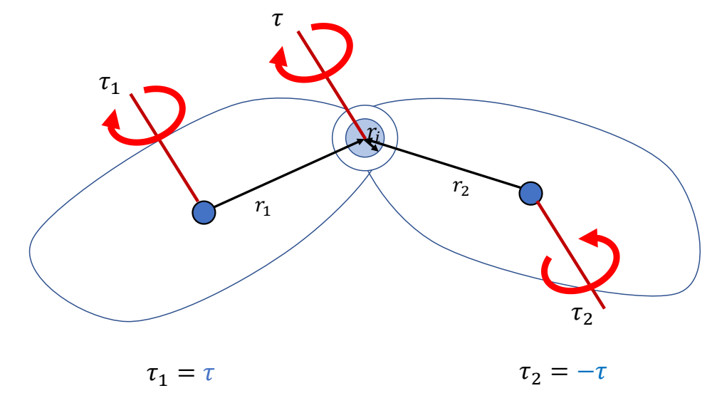
在运动方程中施加关节力矩
两刚体系统
对于两个刚体通过关节连接的系统,运动方程为:
$$ M\begin{bmatrix} \dot{v}_1 \\ \dot{\omega}_1 \\ \dot{v}_2 \\ \dot{\omega}_2 \end{bmatrix} + \begin{bmatrix} 0 \\ \omega_1 \times I_1 \omega_1 \\ 0 \\ \omega_2 \times I_2 \omega_2 \end{bmatrix} = \begin{bmatrix} 0 \\ \tau \\ 0 \\ -\tau \end{bmatrix} + J^T\lambda $$
$$ Jv = 0 $$
| 项 | 含义 |
|---|---|
| $\begin{bmatrix} 0 & \tau & 0 & -\tau \end{bmatrix}^T$ | 关节力矩(主动控制) |
| $J^T\lambda$ | 约束力(被动约束) |
✔ 惯例:通常在子刚体上加 $\tau$,在父刚体上加 $-\tau$。
关节力矩 vs. 约束力
理解关节力矩与约束力的区别是理解角色仿真的关键:
| 特性 | 关节力矩 $\tau$ | 约束力 $J^T\lambda$ |
|---|---|---|
| 来源 | 肌肉收缩、电机驱动 | 关节连接、接触 |
| 方向 | 沿关节轴向 | 由约束条件决定 |
| 计算 | 由控制器生成(如 PD 控制) | 由约束求解器计算 |
| 作用 | 主动驱动运动 | 被动维持约束 |
| 能量 | 可以做功(消耗能量) | 不做功(理想约束) |
关节力矩在控制中的位置
1. 驱动角色运动
关节力矩是角色运动的直接驱动力:
- 行走时腿部关节的力矩
- 抓取时手臂关节的力矩
- 转身时躯干关节的力矩
2. 与肌肉的关系
在生物力学中,关节力矩对应肌肉收缩产生的力矩:
- 伸肌群收缩 → 伸展关节
- 屈肌群收缩 → 弯曲关节
3. 在控制中的位置
$$ \text{控制器} \xrightarrow{\text{生成}} \tau \xrightarrow{\text{仿真}} \text{运动} $$
- PD 控制:根据期望角度和当前角度计算 $\tau$
- 轨迹优化:优化 $\tau$ 序列以实现目标运动
- 强化学习:学习策略网络输出 $\tau$
多刚体系统的关节力矩
对于 $n$ 个刚体、$m$ 个关节的系统:
$$ M\dot{v} + C(x,v) = f_{\text{ext}} + f_{\text{joint}} + J^T\lambda $$
其中 $f_{\text{joint}}$ 是所有关节力矩的堆叠向量。
✔ 关键点:每个关节力矩 $\tau_i$ 只影响其连接的两个刚体,一个加 $\tau_i$,另一个加 $-\tau_i$。
下一步:如何计算关节力矩?
本章介绍了关节力矩是什么,但还有一个关键问题:给定目标状态,如何计算需要的关节力矩 $\tau$?
这将在 Proportional-Derivative Control 中详细讲解。
核心思想(PD 控制): $$ \tau = k_p (\theta_{\text{des}} - \theta_{\text{curr}}) + k_d (\dot{\theta}{\text{des}} - \dot{\theta}{\text{curr}}) $$
| 章节 | 与关节力矩的关系 |
|---|---|
| Proportional-Derivative Control | 如何计算关节力矩 $\tau$ |
| Controlling Characters | PD 控制在角色上的应用 |
| Static Balance | 平衡时的关节力矩计算 |
| Tracking | 优化关节力矩序列跟踪参考运动 |
| Learning | 学习策略输出关节力矩 |
小结
关节力矩的核心要点:
- 物理本质:成对的内力矩,合力为零,合力矩不为零
- 施加方式:在一个刚体上加 $\tau$,另一个加 $-\tau$
- 控制作用:主动驱动角色运动的输入
- 与约束力的区别:$\tau$ 是主动的,$J^T\lambda$ 是被动的
- 与外力的区别:关节力矩只产生旋转,外力产生平动 + 旋转
运动方程的统一形式: $$ M\dot{v} + C(x,v) = f_{\text{ext}} + f_{\text{joint}} + J^T\lambda $$
$$ Jv = 0 $$
本文出自 CaterpillarStudyGroup,转载请注明出处。 https://caterpillarstudygroup.github.io/GAMES105_mdbook/
运动方程中的力与力矩
✅ 本章定位:澄清物理仿真运动方程中 力 和 力矩 的来源与含义。
一、力与力矩的作用效果
施加力/力矩会得到的效果
| 力加在质心上,只会导致平移,不会导致旋转。 |  |
| ✂ 在物体边缘施加力,等价于在质心施加力,并施加一个导致旋转的力矩。 | 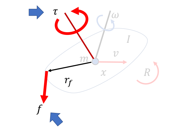 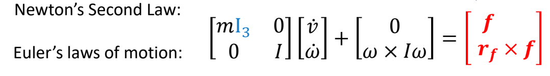 |
| ✂ 在质心上施加一个力矩,等价于施加一对大小相同方向相反的力。在质心处的合力为零,不会产生位移,只会产生旋转。 ✂ 力矩只是数学上的概念。 | 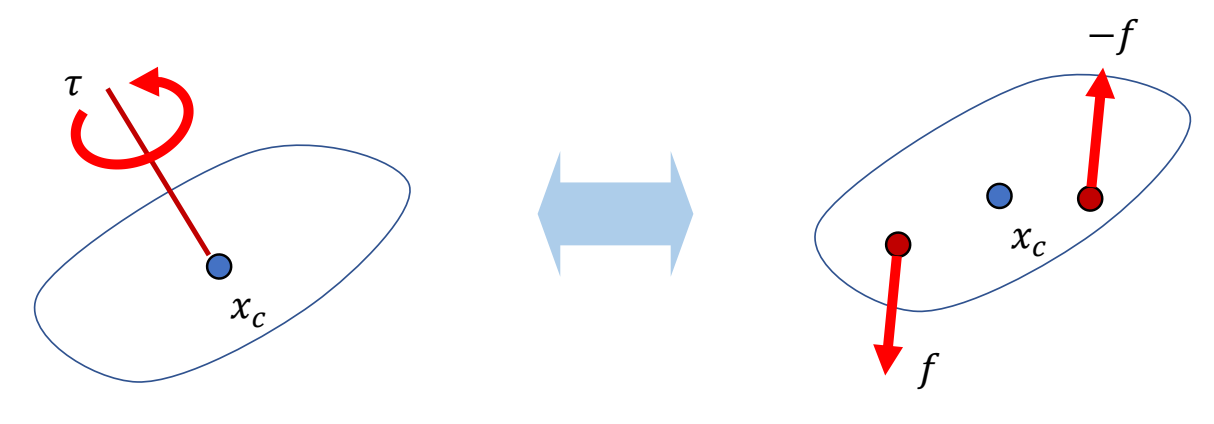 |
怎么对角色产生效果
✂ 想让角色做指定动作,不能直接修改其状态,而是控制力影响状态。
| ✂ 为了驱动角色,可以单独对每个刚体施加力或力矩。 | 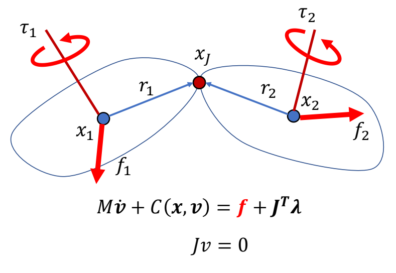 |
| ✂ 也可以在关节上施加力矩。 | 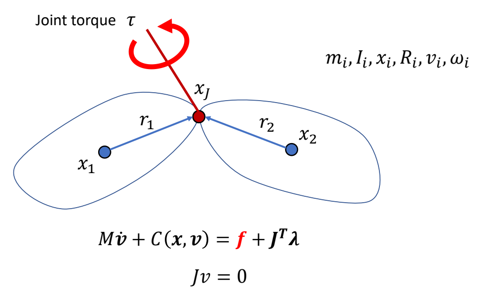 |
✂ 回顾前面公式,力和力矩都是施加在刚体上的,如何施加在关节上?
二、运动方程回顾
对于有 \(n\) 个刚体、\(m\) 个关节的角色系统,运动方程为:
$$ M\dot{v} + C(x,v) = f_{\text{ext}} + f_{\text{joint}} + J^T\lambda $$
$$ Jv = 0 $$
方程中有三个力/力矩项,它们的来源和含义完全不同:
| 项 | 名称 | 来源 | 是否主动 |
|---|---|---|---|
| \(f_{\text{ext}}\) | 外力 | 外部环境 | 被动 |
| \(f_{\text{joint}}\) | 关节力矩 | 控制器 | 主动 |
| \(J^T\lambda\) | 约束力 | 约束求解器 | 被动 |
三、外力 (f_{\text{ext}})
定义
外力 是来自角色外部的力,包括:
| 外力类型 | 说明 | 计算公式 |
|---|---|---|
| 重力 | 地球引力 | \(f_g = m \cdot g\) |
| 风力 | 环境气流 | 经验模型 |
| 接触力 | 地面/物体的支撑力 | 由接触模型计算 |
| 摩擦力 | 接触面的切向阻力 | \(f_t = -\mu f_n \frac{v_{\parallel}}{|v_{\parallel}|}\) |
外力的效果
外力作用在刚体上,会同时产生两种效果:
     外力 f
       ↓
   ┌───────┐
   │ 刚体  │ ← 质心
   └───────┘
       ↑
      r (作用点距离质心)
平移效果(无论作用在哪里): $$ a = \frac{f_{\text{ext}}}{m} $$
旋转效果(仅当不经过质心时): $$ \tau_{\text{ext}} = r \times f_{\text{ext}} $$
✅ 关键:外力产生的力矩 \(\tau_{\text{ext}}\) 已经包含在 \(f_{\text{ext}}\) 中,不需要单独列一项。
重要性质
| 性质 | 说明 |
|---|---|
| 被动性 | 外力不由控制器决定,由物理环境决定 |
| 无控制器时仍存在 | Ragdoll 只受外力,也会运动 |
| 力矩在 \(f_{\text{ext}}\) 中 | 外力不经过质心产生的力矩,算在 \(f_{\text{ext}}\) 里 |
四、关节力矩 (f_{\text{joint}})
定义
关节力矩 是控制器生成的主动控制输入,用于驱动角色运动:
$$ f_{\text{joint}} = \begin{bmatrix} 0 & \tau_1 & 0 & -\tau_1 & \cdots \end{bmatrix}^T $$
来源
| 来源 | 说明 |
|---|---|
| 肌肉收缩 | 生物角色的肌肉产生力矩 |
| 电机驱动 | 机器人关节的电机产生力矩 |
| 控制器输出 | PD 控制、强化学习策略等 |
施加方式
关节力矩 \(\tau\) 作用在关节连接的两个刚体上:
        τ (子刚体)
    ┌────┐
    │前臂│  ← 子刚体
    └────┘
       ↖
      手肘关节
    ┌────┐
    │上臂│  ← 父刚体
    └────┘
       -τ (父刚体)
规则:
- 在子刚体上加 \(\tau\)
- 在父刚体上加 \(-\tau\)
- 合力为零:\(\tau + (-\tau) = 0\)(满足牛顿第三定律)
关节力矩的效果
关节力矩只产生纯旋转,不产生平移:
$$ \alpha = I^{-1}\tau $$
✅ 与外力的区别:外力同时产生平动和转动,关节力矩只产生转动。
重要性质
| 性质 | 说明 |
|---|---|
| 主动性 | 由控制器主动生成 |
| 无控制器时为零 | Ragdoll 的 \(f_{\text{joint}} = 0\) |
| 不在 \(f_{\text{ext}}\) 中 | 关节力矩是独立项 |
| 外力不产生关节力矩 | 即使外力不经过质心,产生的力矩也在 \(f_{\text{ext}}\) 中,不在 \(f_{\text{joint}}\) 中 |
五、两种力矩的对比
外力产生的力矩 vs. 关节力矩
| 维度 | 外力产生的力矩 \(\tau_{\text{ext}}\) | 关节力矩 \(\tau_{\text{joint}}\) |
|---|---|---|
| 来源 | 外力不经过质心 | 控制器生成 |
| 在方程中的位置 | \(f_{\text{ext}}\) 中(通过 \(r \times f\) 计算) | \(f_{\text{joint}}\) 中 |
| 是否需要控制器 | 否(Ragdoll 也有) | 是(无控制器则为 0) |
| 物理本质 | 被动力矩 | 主动控制输入 |
| 例子 | 重力让手臂自然下垂 | 主动抬手 |
直观类比
| 场景 | 力矩来源 | 在方程中的位置 |
|---|---|---|
| 风吹门 | 风力不经过质心 | \(f_{\text{ext}}\) |
| 你推门 | 手施加的力矩 | \(f_{\text{joint}}\) |
六、无控制器时的情况(Ragdoll)
运动方程
当没有控制器时:
$$ f_{\text{joint}} = 0 $$
方程简化为:
$$ M\dot{v} + C(x,v) = f_{\text{ext}} + J^T\lambda $$
为什么 Ragdoll 的关节会旋转?
即使 \(f_{\text{joint}} = 0\),Ragdoll 仍然会运动,原因是:
- 外力(重力)作用在每个刚体上
- 外力不经过质心时产生力矩(在 \(f_{\text{ext}}\) 中)
- 关节约束限制刚体不分离,但允许绕关节旋转
- 结果:刚体绕关节被动旋转
被动旋转 vs. 主动旋转
| 旋转类型 | 来源 | 方程中的项 | 例子 |
|---|---|---|---|
| 被动旋转 | 外力产生的力矩 | \(f_{\text{ext}}\) | Ragdoll 倒下、手臂自然摆动 |
| 主动旋转 | 关节力矩 | \(f_{\text{joint}}\) | 主动抬手、走路摆臂 |
七、总结
关键要点
-
\(f_{\text{ext}}\)(外力):
- 来自外部环境(重力、风力、接触力)
- 包含外力产生的力矩(\(r \times f\))
- 无控制器时仍然存在
-
\(f_{\text{joint}}\)(关节力矩):
- 来自控制器(肌肉、电机)
- 只包含控制器主动生成的力矩
- 不包含外力产生的力矩
- 无控制器时为零
-
外力产生的力矩永远在 \(f_{\text{ext}}\) 中,与 \(f_{\text{joint}}\) 无关。
一张表理解
$$ \begin{array}{c|c|c} \text{项} & \text{包含什么} & \text{无控制器时} \ \hline f_{\text{ext}} & \text{外力 + 外力产生的力矩} & \text{仍然存在} \ f_{\text{joint}} & \text{仅控制器生成的关节力矩} & 0 \ J^T\lambda & \text{约束力求解结果} & \text{仍存在(维持约束)} \ \end{array} $$
本文出自 CaterpillarStudyGroup,转载请注明出处。 https://caterpillarstudygroup.github.io/GAMES105_mdbook/
八、前向动力学与后向动力学
Forward Dynamics vs. Inverse Dynamics
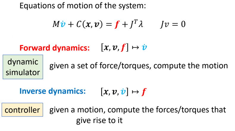
✂ 运动方程,本质上是建立力与加速度之间的联系。 ✂ 前向与后向,是一个运动方程的两种用法。 ✂ 仿真器为前向部分,控制器为逆向部分。
前向动力学(Forward Dynamics)
已知:力/力矩 \(f, \tau\)
求解:加速度 \(\dot{v}\)
$$ \dot{v} = M^{-1}(f_{\text{ext}} + f_{\text{joint}} + J^T\lambda - C(x,v)) $$
用途:
- 物理仿真器
- 给定控制输入,预测角色会如何运动
后向动力学(Inverse Dynamics)
已知:加速度 \(\dot{v}\)(期望的运动)
求解:力/力矩 \(f, \tau\)
$$ f_{\text{joint}} = M\dot{v} + C(x,v) - f_{\text{ext}} - J^T\lambda $$
用途:
- 控制器设计
- 给定目标运动,计算需要的关节力矩
对比
| 前向动力学 | 后向动力学 | |
|---|---|---|
| 已知 | 力/力矩 | 加速度(期望运动) |
| 求解 | 加速度 | 力/力矩 |
| 用途 | 仿真器 | 控制器 |
| 问题类型 | 正向问题 | 逆向问题 |
✅ 关键:前向和后向是同一个运动方程的两种用法,只是已知量和求解量不同。
Contacts
✔ 如何处理与地面的接触,让人站在地面上。
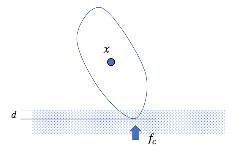
✔ 要解决的问题:
- 地面接触检测:检测哪些点/面与地面接触
- 接触力施加:如何对碰撞点施加力,使物体不陷入地面
💡 与 GAMES103 的分工
- GAMES103 - 碰撞检测与响应:详细介绍碰撞检测算法(Broad Phase、Narrow Phase、GJK、CCD)和穿透解除方法(内点法、Impact Zone)
- GAMES105 - 接触约束求解:focus 在如何将接触建模为约束,并与关节约束统一求解
深入学习:
方法一:Penalty-based Contact Model(基于惩罚的接触模型)
基本思想
用弹簧 - 阻尼模型近似接触力:当物体穿透地面时,产生一个与穿透深度成正比的斥力。
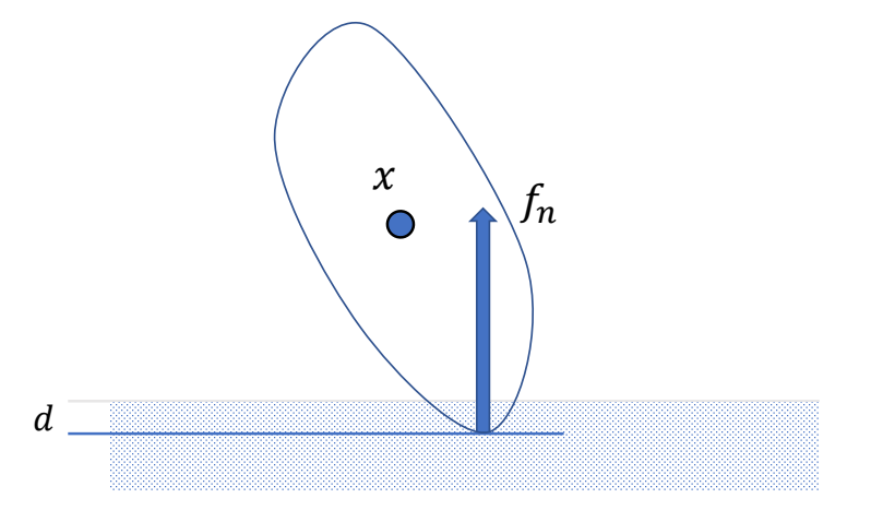
$$ f_n = -k_p d - k_d v_{c,\perp} $$
| 参数 | 含义 |
|---|---|
| $d$ | 穿透深度($d > 0$ 时公式生效) |
| $k_p$ | 弹簧刚度(越大越不容易穿透) |
| $k_d$ | 阻尼系数(防止反弹) |
| $v_{c,\perp}$ | 接触点法向速度 |
✔ 效果:会有一些陷入,但不会陷入太多 ❐ 支持力竟然不是 $-mg$,而是由弹簧模型决定
考虑摩擦力
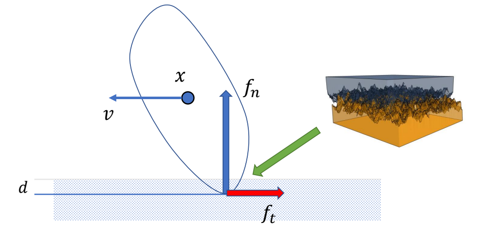
动摩擦力模型: $$ f_t = -\mu f_n \frac{v_{c,\parallel}}{||v_{c,\parallel}||} $$
| 参数 | 含义 |
|---|---|
| $\mu$ | 摩擦系数 |
| $f_n$ | 法向支持力 |
| $v_{c,\parallel}$ | 接触点切向速度 |
✔ 一般不模拟静摩擦力
存在的问题
| 问题 | 原因 | 后果 |
|---|---|---|
| $k_p$ 必须很大 | 否则脚陷地明显 | 需要非常小的时间步长 |
| $k_d$ 必须非常大 | 否则地面像蹦床 | 数值不稳定 |
| 时间步长必须小 | 高增益导致刚度大 | 仿真效率低 |
💡 与 GAMES103 内点法的关系
GAMES103 中介绍的**内点法(Interior Point Methods)**使用了类似的惩罚思想,但用能量场定义斥力:
$$ E(\mathbf{x}) = -\rho \log ||\mathbf{x}_{ij}|| $$
$$ \mathbf{f} = -\nabla E = \rho \frac{\mathbf{x}{ij}}{||\mathbf{x}{ij}||^2} $$
两种方法本质相同:距离越近,斥力越大。GAMES105 使用简化的弹簧模型,更易于理解。
方法二:Contact as a Constraint(接触作为约束)
✔ 另一种方法,把接触建模为数学约束,与关节约束统一求解。
接触点状态分析
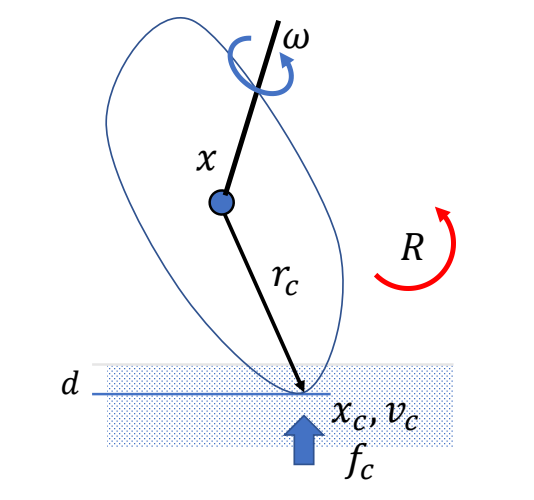
接触点 $x_c$ 的位置表示: $$ x_c = x + r_c $$
接触点 $x_c$ 的速度表示: $$ v_c = v + \omega \times r_c = J_c \begin{bmatrix} v \\ \omega \end{bmatrix} $$
接触点法向速度: $$ v_{c,\perp} = J_{c,\perp} \begin{bmatrix} v \\ \omega \end{bmatrix} $$
接触点约束分析
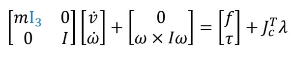
✔ 约束 1:点在竖直方向的速度必须 $\geq 0$,即只能向上移动(不能向下穿透)。
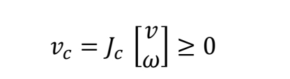
✔ 约束 2:力的大小 $\lambda > 0$,只能推,不能拉。$\lambda$ 是力与速度的大小比例系数。

✔ 约束 3:力和速度只能有一个不为零,否则会做功(互补条件)。
$$ v_c \perp \lambda = 0 $$
线性互补问题(LCP)
✔ 合在一起称为线性互补方程,是碰撞建模的标准方式。
这类问题被称为:(Mixed) Linear Complementary Problem (LCP)
解 LCP 的方法有:
- Lemke's algorithm – a simplex algorithm
- Projected Gauss-Seidel
- 其他数值优化方法
❐ 这个方程比较难解,计算成本高于 Penalty 方法
考虑摩擦力的约束问题
How to deal the friction?
🔍 推荐阅读:Fast contact force computation for nonpenetrating rigid bodies. David Baraff. SIGGRAPH '94
✔ 该论文提出了快速实现静摩擦约束的建模方法。
两种方法对比
| 特性 | Penalty-based | Constraint-based (LCP) |
|---|---|---|
| 原理 | 弹簧 - 阻尼模型近似 | 数学约束精确建模 |
| 穿透 | 允许少量穿透 | 无穿透 |
| 求解 | 直接计算力 | 需要专门求解器 |
| 计算成本 | 低 | 高 |
| 数值稳定性 | 需要小步长 | 较稳定 |
| 与关节约束统一 | 否 | ✅ 是 |
| 适用场景 | 实时应用、游戏 | 精确仿真、研究 |
在运动方程中的位置
对于有接触的角色系统,运动方程为:
$$ M\dot{v} + C(x,v) = f_{\text{ext}} + f_{\text{joint}} + J_{\text{contact}}^T \lambda_{\text{contact}} $$
$$ J_{\text{contact}} v \geq 0, \quad \lambda_{\text{contact}} \geq 0, \quad (J_{\text{contact}} v) \perp \lambda_{\text{contact}} $$
✔ 关键:接触约束与关节约束形式统一,可以同时求解!
本文出自 CaterpillarStudyGroup,转载请注明出处。 https://caterpillarstudygroup.github.io/GAMES105_mdbook/
仿真流程总结
✅ 本章定位:串联整个物理仿真章节,展示完整的仿真 Pipeline。
💡 前置知识:关于角色的分段刚体表示,见 RigidBodyRepresentation.md
完整仿真 Pipeline

✅ 角色仿真的完整流程:
- 计算当前状态 - 位置、速度、约束信息
- 计算外力 - 重力、风力、关节力矩(由控制器生成)
- 检测约束 - 关节约束、接触约束
- 求解约束力 - 解出 \(\lambda\),计算 \(J^T\lambda\)
- 积分更新状态 - 更新位置、速度
仿真方程
分段多刚体系统(详见 RigidBodyRepresentation.md):
$$ M\dot{v} + C(x,v) = f + J^T\lambda $$
| 项 | 含义 | 对应章节 |
|---|---|---|
| \(M\dot{v} + C(x,v)\) | 惯性力 | RigidBodyRepresentation.md |
| \(f\) | 外力 | 重力、风力、关节力矩 |
| \(J^T\lambda\) | 约束力 | Constraints.md / JointConstraint.md / Contacts.md |
仿真流程详解
步骤 1:计算外力
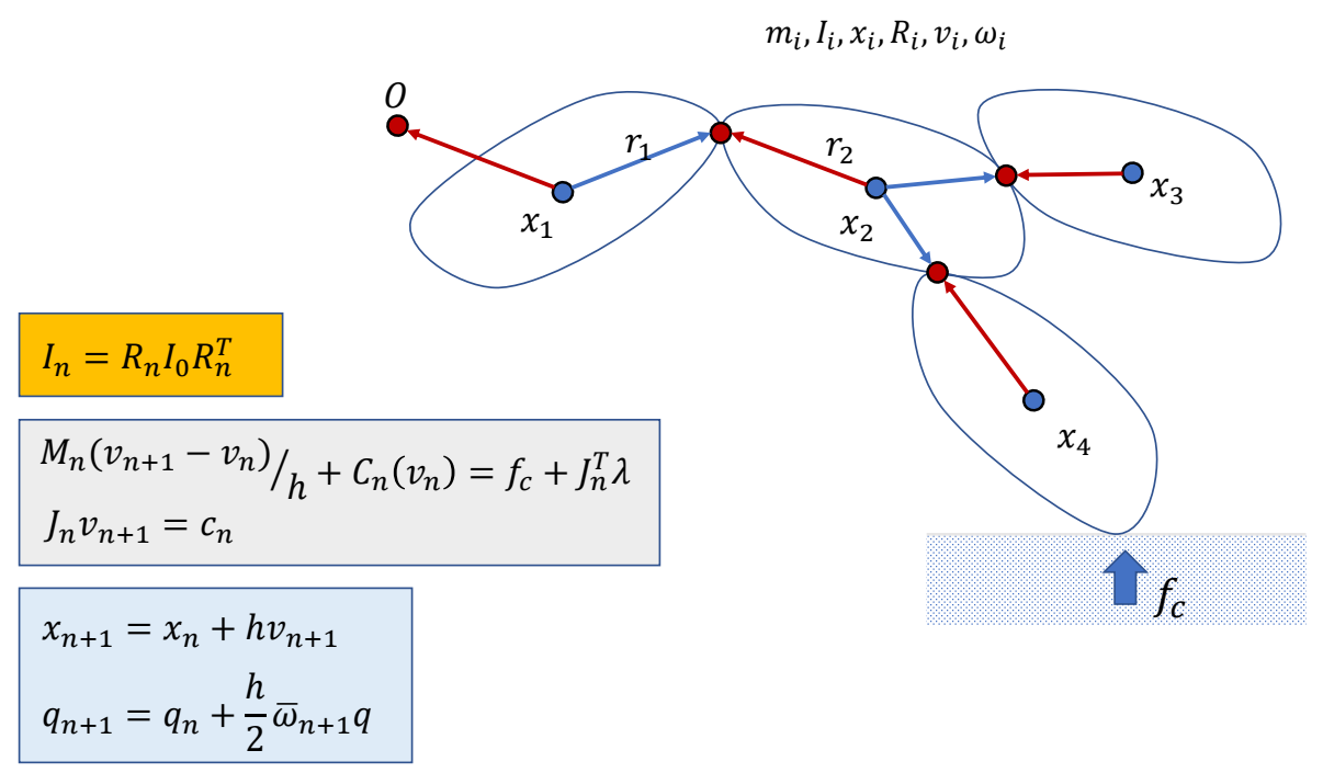
✅ 外力包括:
- 重力:\(mg\)
- 风力等其他外力
- 关节力矩:由控制器(如 PD 控制)生成
步骤 2:约束求解
关节约束(详见 JointConstraint.md):
- 防止刚体分离
- 求解 \(J^T\lambda\)
接触约束(详见 Contacts.md):
- 防止穿透地面
- 摩擦力防止滑动
步骤 3:积分更新
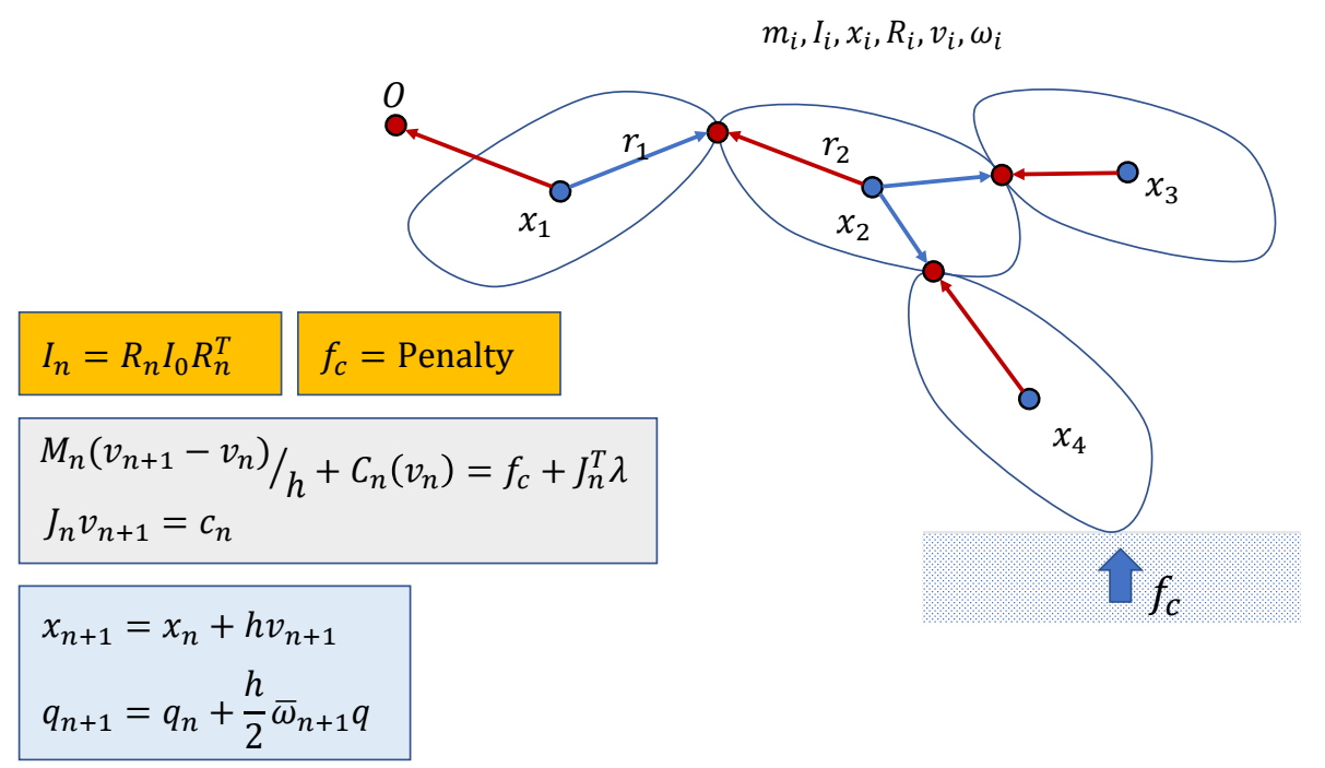
✅ 把人简化为分段刚体。整体过程为:
- (1) 黄:计算当前状态
- (2) 绿:计算约束,求解,解出下一时刻的速度
- (3) 蓝:更新下一时刻的量(积分)
本章小结
| 章节 | 内容 |
|---|---|
| Simulation.md | 仿真器概述、力与力矩、前向/后向动力学 |
| RigidBodyRepresentation.md | 角色的分段刚体表示 |
| Constraints.md | 约束求解原理(小球例子) |
| JointConstraint.md | 关节约束与关节力矩 |
| Contacts.md | 接触模型 |
| 本文 | 完整仿真流程总结 |
核心公式: $$ M\dot{v} + C(x,v) = f + J^T\lambda $$
本文出自 CaterpillarStudyGroup,转载请注明出处。 https://caterpillarstudygroup.github.io/GAMES105_mdbook/
PD 控制
✅ 本章定位:理解如何设计和应用 PD 控制器,将目标状态转换为关节力矩。
在控制系统中的位置
flowchart TD
    subgraph "高层:任务规划"
        A["做什么动作?<br/>有限状态机、行为树"]
    end

    subgraph "中层:轨迹生成/策略学习"
        B["如何生成目标动作?<br/>轨迹优化、DeepMimic、AMP"]
    end

    subgraph "底层:执行控制 (本章)"
        C["如何计算关节力矩?<br/>PD 控制"]
    end

    subgraph "仿真器"
        D["物理仿真<br/>Mv̇ + C = f + Jᵀλ"]
    end

    A -->|动作指令 | B
    B -->|目标状态 q*, q̇* | C
    C -->|关节力矩 τ | D
    D -->|当前状态 q, q̇ | C
    D -->|新状态 | A
| 层次 | 功能 | 典型方法 |
|---|---|---|
| 高层 | 任务规划:决定做什么动作 | 有限状态机、行为树 |
| 中层 | 轨迹生成:输出目标状态 \(q^, \dot{q}^\) | 轨迹优化、DeepMimic、AMP |
| 底层 | 执行控制:计算关节力矩 \(\tau\) | PD 控制 |
PD 控制的输入输出:
- 输入:目标状态 \(q^, \dot{q}^\) + 当前状态 \(q, \dot{q}\)
- 输出:关节力矩 \(\tau\) → 送入仿真器
与仿真器的关系
| 模块 | 输入 | 输出 | 核心问题 |
|---|---|---|---|
| 控制器 | 目标状态/轨迹 + 当前状态 | 关节力矩 τ | 如何生成力矩让角色达到目标? |
| 仿真器 | 关节力矩 τ + 外力 | 新状态 | 给定力矩,角色会如何运动? |
分工说明:
- 控制器是「逆向问题」:从目标反推力矩
- 仿真器是「前向问题」:从力矩推算运动
✅ 详细讲解见 角色物理仿真基础
本章内容导航
| 文件 | 内容 |
|---|---|
| 关节力矩 | 什么是关节力矩 - 物理定义与数学推导 - 为什么需要关节力矩(vs. 外力) - 在运动方程中的位置 |
| Proportional-Derivative Control | PD 控制理论基础 - 简化例子:物体上下移动 - P 控制、PD 控制、PID 控制 - Stable PD(隐式欧拉) |
| Controlling Characters | PD 在角色上的应用 - 参数调优(\(k_p\)、\(k_d\)) - 欠驱动问题与净外力 - 稳态误差问题 |
| Static Balance | 静态平衡专题 - 支撑面与质心 - PD 控制策略 - Jacobian Transpose Control |
本章重点问题
-
PD 参数如何调优?
- \(k_p\) 太小:无法达到目标
- \(k_p\) 太大:角色僵硬
- \(k_d\) 太小:振荡
- \(k_d\) 太大:响应慢
-
欠驱动系统如何处理?
- 人形角色是欠驱动系统(无法直接控制质心位置)
- 解决方案:净外力(root force/torque)
-
稳态误差如何解决?
- PD 控制需要误差才能产生力
- 解决方案:增大 \(k_p\) 或使用前馈补偿
-
如何保证数值稳定性?
- 高增益需要小时间步长
- 解决方案:隐式欧拉(Stable PD)
补充概念
Fully-Actuated vs. Underactuated
在上一节中,\(f\) 与 \(V\) 的自由度可能是不同的。\(f\) 是关节数\( × 3\),\(V\) 是刚体数\( × 3\)。
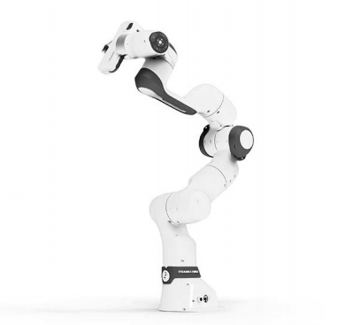 | 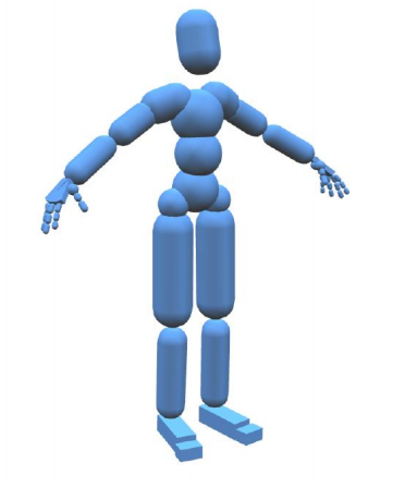 |
| If #actuators ≥ #dofs, the system is fully-actuated | If #actuators < #dofs, the system is underactuated |
| For any \([x,v,\dot{v} ]\), there exists an \(f\) that produces the motion | For many \([x,v,\dot{v} ]\) , there is no such \(f\) that produces the motion |
| ✅ 可以精确控制机械臂到达目标状态。 | ✅ 不借助外力情况,人无法控制 Hips 的状态(位置)。 |
✅ #actuators:\(f \) 和 \(\tau \) 的自由度。 ✅ #dofs:角色状态的自由度。 ✅ 避免让角色掉入无法控制的状态。
✅ 深入学习:欠驱动系统问题 - 详细讲解人形角色为什么是欠驱动系统以及解决方案。
Feedforward vs. Feedback
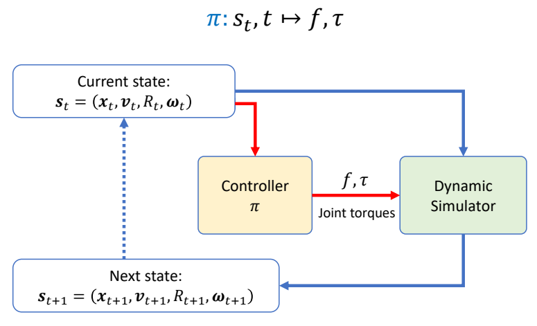
驱动角色运动的控制器是通过优化目标函数产生的。
| Feedforward control | Feedback control |
|---|---|
| \(f,\tau =\pi (t)\) | \(f,\tau =\pi (s_t,t)\) |
| Apply predefined control signals without considering the current state of the system | Adjust control signals based on the current state of the system |
| Assuming unchanging system. | Certain perturbations are expected. |
| Perturbations may lead to unpredicted results ✅ 如果角色受到挠动而偏离了原计划,无法修正回来。 | The feedback signal will be used to improves the performance at the next state. |
P55
Proportional-Derivative Control
这是一种常用的控制器。
✅ 有反馈,但还是算是前向控制,因为反馈的部分和想控制的部分不完全一致。
这一页先用一个简化问题来分析PD控制
问题描述
Compute force \(f\) to move the object to the target height
✅ 例子:物体只能沿竿上下移动,且受到重力。
✅ 控制目的:设计控制器,使物体在控制力的作用下达到目标高度。
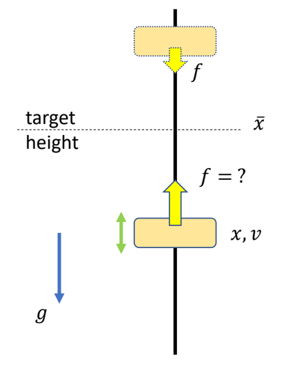
使用比例控制
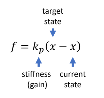
实际上:会产生上下振荡,不会停在目标位置。
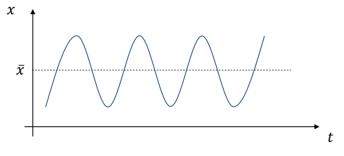
P56
比例控制+Damping
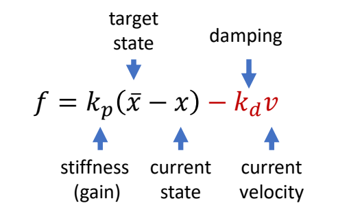
✅ 改进:如果物体已有同方向速度,则力加得小一点。
P57
比例微分控制
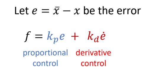
✅ 第一项:比例控制;第二项:微分控制
P59
✅ 存在的问题:为了抵抗重力,一定会存在这样的误差。
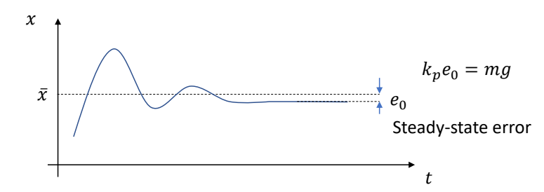
P60
Increase stiffness \(k_p\) reduces the steady-state error, but can make the system too stiff and numerically unstable
✅ 增加 \(k_p\) 可以减小误差,但会让人看起来很僵硬。
P61
比例积分微分控制 Proportional-Integral-Derivative controller
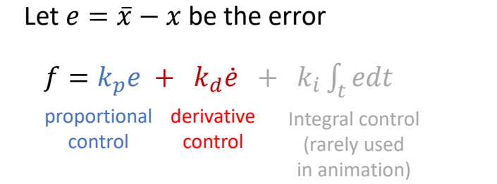
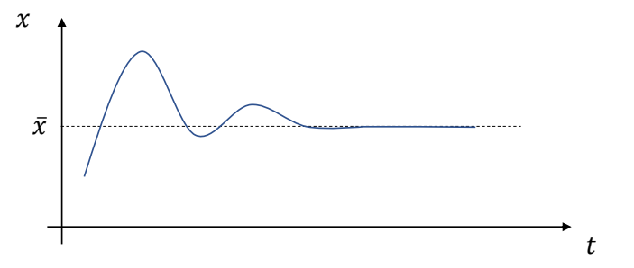
✅ 解决误差方法:积分项。
✅ 但角色动画通常不用积分项。
✅ 积分项跟历史相关,会带来实现的麻烦和控制的不稳定。
Stable PD Control
✅ PD control 的过程类似于一个弹簧系统。
✅ 因此利用弹簧系统中的半隐式欧拉来提升 PD 的稳定性。
显式欧拉的PD控制的稳定性分析
✅ \(h\) 为时间步长。
✅ (1) 假设 \(m=1\) (2) 代入 \(f\) 到方程组 (3) 方程组写成矩阵形式,得:
P11
$$ \begin{bmatrix} v_{n+1}\\ x_{n+1} \end{bmatrix}=\begin{bmatrix} 1-k_dh & -k_ph\\ h(1-k_dh) & 1-k_ph^2 \end{bmatrix}\begin{bmatrix} v_n \\ x_n \end{bmatrix} $$
P14
提取常数方程A,得:
$$ A=\begin{bmatrix} 1-k_dh & -k_ph\\ h(1-k_dh) & 1-k_ph^2 \end{bmatrix} $$
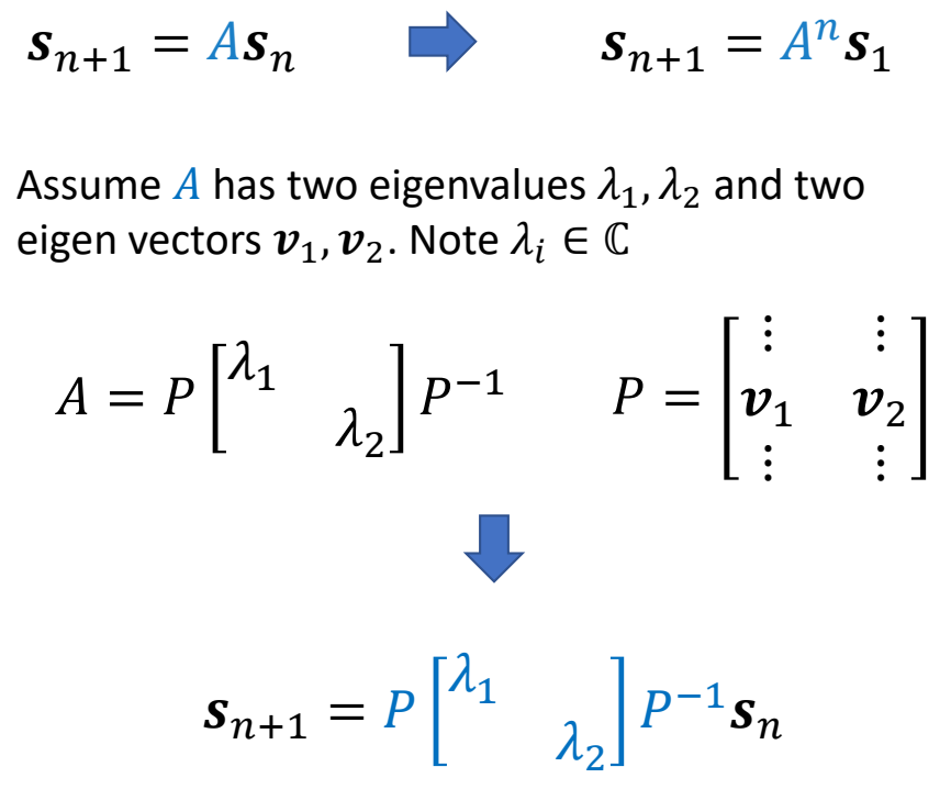
\(\lambda _1,\lambda _2 \in \mathbb{C} \) are eigenvalues of \(A\)
✅ 基于中间变是 \(z_n\) 推导的过程跳过。
✅ 根据矩阵特征值的性质可直接得出结论。
if \(|\lambda _1|> 1\)
The system is unstable!
Condition of stability: \(|\lambda _i|\le 1 \text{ for all } \lambda _i\)
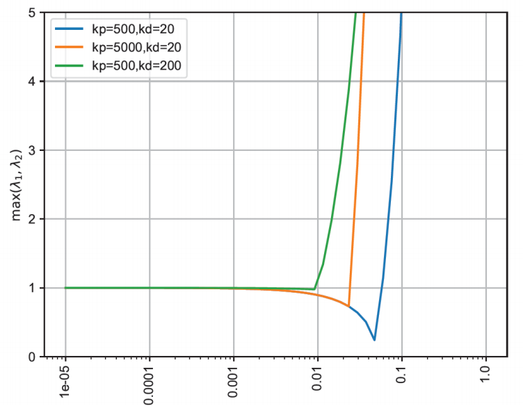
✅ 如果 \(k_p\) 和 \(k_d\) 变大,就必须以一个较小的时间步长进行仿真。
P22
隐式欧拉的PD控制
✅ 解决方法:半隐式欧拉 → 隐式欧拉,即用下一时刻的力计算下一时刻的速度。
- 半隐式欧拉
$$ \begin{align*} v_{n+1} & = v_n+h(-k_px_n-k_dv_n) \\ v_{n+1} & = x_n+hv_{n+1} \end{align*} $$
$$ \Downarrow $$
- 隐式欧拉
$$ \begin{align*} v_{n+1} & = v_n+h(-k_px_n-k_dv_{n+1}) \\ x_{n+1} & = x_n+hv_{n+1} \end{align*} $$
✅ 实际上,计算 \(f_{n+1}\) 只使用 \(V_{n+1}\) , 不使用 \(x_{n+1}\) , 因为 \(x_{n+1}\) 会引入非常复杂的计算。
✅ 由于 \(v_{n+1}\) 未知,需通过解方程组来求解。
P23
得到的方程组为:
$$ \begin{bmatrix} v_{n+1} \\ x_{n+1} \end{bmatrix}=\frac{1}{1+hk_d} \begin{bmatrix} 1 & -k_ph\\ h & 1+k_dh-k_ph^2 \end{bmatrix}\begin{bmatrix} v_n\\ x_n \end{bmatrix} $$

✅ \(v_{n}\) 换成 \(v_{n+1}\) ,很大承度上提高了稳定性。
本文出自CaterpillarStudyGroup,转载请注明出处。
https://caterpillarstudygroup.github.io/GAMES105_mdbook/
P3
PD Control for Characters
✅ 前面是 PD 的例子,这里是 PD 在物理仿真角色上的应用,计算在每个关节上施加多少力矩。
控制系统层次:PD 控制属于底层执行控制,输入是目标关节位置 $q^$ 和速度 $\dot{q}^$,输出是关节力矩 $\tau$。
中层策略:轨迹优化或 DeepMimic/AMP/ASE 等学习方法输出 PD 的目标 $q^*$。
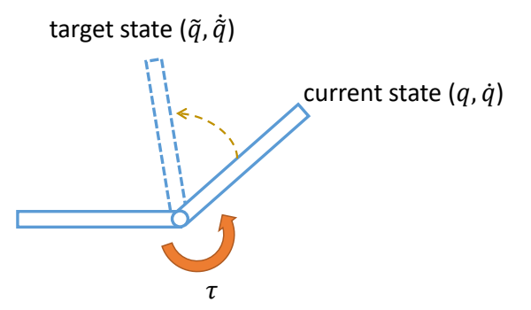
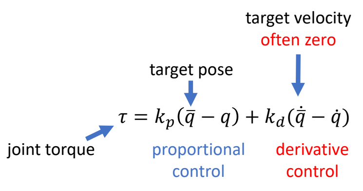
✅ 通常目标的速度 \(\dot{\bar{q}} = 0\).
因此:
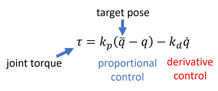
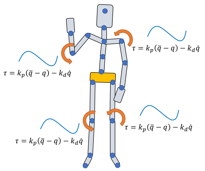
P63
PD Control for Characters 的参数和效果
✅ \(K_p\) 太小:可能无法达到目标状态。 ✅ \(K_p\) 太大:人体很僵硬。 ✅ \(k_d\) 太小:动作有明显振荡。 ✅ \(k_d\) 太大,要花更多时间到达目标资态。
-
Determining gain and damping coefficients can be difficult…
- A typical setting \(k_p\) = 200, \(k_d\) = 20 for a 50kg character
- Light body requires smaller gains
- Dynamic motions need larger gains
-
High-gain/high-damping control can be unstable, so small times is necessary
- \(h\) = 0.5~1ms is often used, or 1000~2000Hz
- \(h\) = 1/120s~1/60s, or 120Hz/60Hz with Stable PD
- Higher gain/damping requires smaller time step
P66
P72
欠驱动系统问题
✅ 详细说明:参见 欠驱动系统问题
由于是欠驱动系统,Tracking Mocap with Joint Torques 会遇到问题,因为:
- \(\tau _j\): joint torques
- Apply \(\tau _j\) to "child" body
- Apply \(-\tau _j\) to "parent" body
- All forces/torques sum up to zero
✅ 合力为零,无法控制整体的位置和朝向。 ✅ 解决方法:增加净外力(Root Force/Torque),详见 欠驱动系统问题
稳态误差问题
✅ 详细说明:参见 稳态误差问题
PD control computes torques based on errors
Steady state error
This arm never reaches the target angle under gravity

在角色上的表现就是 Motion falls behind the reference
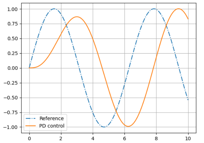
✅ 核心问题:需要有误差才能计算 force,有了 force 才能控制。 ✅ 解决方法:增大 \(k_p\)、Stable PD、前馈补偿,详见 稳态误差问题
前馈控制 vs. 反馈控制
✅ 详细说明:参见 前馈与反馈控制
Is PD control a feedforward control? a feedback control?
答案:取决于观察层次
| 观察层次 | 控制类型 | 原因 |
|---|---|---|
| 关节级别 | 反馈控制 | 使用当前关节状态 \(q\) 计算力矩 |
| 系统级别 | 前馈控制 | 目标状态由上层决定,PD 只是执行器 |
✅ 深入学习:前馈与反馈控制 - 详细讲解两者的区别、组合控制方案、以及在 DeepMimic/AMP 中的应用。
本文出自 CaterpillarStudyGroup,转载请注明出处。
https://caterpillarstudygroup.github.io/GAMES105_mdbook/
欠驱动系统问题(Underactuated System)
✅ 本章定位:理解人形角色为什么是欠驱动系统,以及 PD 控制如何处理这个问题。
一、什么是欠驱动系统
定义
| Fully-Actuated(完全驱动) | 执行器数量 \(\geq\) 自由度数量 |
| Underactuated(欠驱动) | 执行器数量 \(<\) 自由度数量 |
数学表述:
$$ f, \tau \text{ 的自由度} < V \text{ 的自由度} $$
其中:
- \(f, \tau\):可主动控制的力/力矩
- \(V\):角色状态的自由度
二、人形角色为什么是欠驱动系统
自由度分析
对于一个人形角色:
| 自由度类型 | 数量 | 是否可直接控制 |
|---|---|---|
| 根节点位置(Hips) | 3 平移 + 3 旋转 = 6 | ❌ 不可直接控制 |
| 关节旋转 | 约 30+ | ✅ 可通过 \(\tau\) 控制 |
关键问题
无法直接控制质心位置:
     关节力矩 τ
        ↓
    只能控制关节旋转
        ↓
    无法直接控制 Hips 位置
        ↓
    需要借助外力(地面反作用力)
三、欠驱动带来的控制挑战
问题 1:无法直接控制质心
场景:想让角色向前走
❌ 错误思路:
   直接控制 Hips 向前移动 → 做不到!

✅ 正确思路:
   1. 用关节力矩 \\(\tau\\) 驱动腿部关节
   2. 脚对地面施加力
   3. 地面反作用力推动质心向前
问题 2:PD 控制的局限性
PD 控制公式:
$$ \tau = k_p (\theta_{\text{des}} - \theta_{\text{curr}}) + k_d (\dot{\theta}{\text{des}} - \dot{\theta}{\text{curr}}) $$
局限性:
- PD 控制只能控制关节角度
- 无法直接控制质心位置
- 质心运动是关节运动的间接结果
四、与完全驱动系统的对比
完全驱动系统(如机械臂)
     基座固定
        ↓
   所有关节都可控
        ↓
   可直接控制末端执行器位置
| 特性 | 机械臂(完全驱动) | 人形角色(欠驱动) |
|---|---|---|
| 基座 | 固定 | 自由浮动 |
| 可控自由度 | 所有关节 | 仅关节旋转 |
| 质心控制 | 间接 | 间接(需外力) |
欠驱动 vs. 完全驱动
| |
| If #actuators \(\geq\) #dofs, the system is fully-actuated | If #actuators \(<\) #dofs, the system is underactuated |
| For any \([x,v,\dot{v}]\) , there exists an \(f\) that produces the motion | For many \([x,v,\dot{v}]\) , there is no such \(f\) that produces the motion |
| ✅ 可以精确控制机械臂到达目标位置。 | ✅ 不借助外力情况,人无法控制 Hips 的位置。 |
✅ #actuators:\(f\) 和 \(\tau\) 的自由度。 ✅ #dofs:角色状态的自由度。
五、解决方案
方案 1:净外力(Root Force/Torque)
核心思想:在根节点(Hips)上施加虚拟的力和力矩。
$$ \tau_{\text{root}} = k_p (x_{\text{des}} - x_{\text{curr}}) + k_d (\dot{x}{\text{des}} - \dot{x}{\text{curr}}) $$
说明:
- 虚拟力,不真实存在
- 用于计算期望的地面反作用力
- 在优化框架中常用
方案 2:动量控制(Momentum Control)
核心思想:通过控制动量来间接控制质心。
$$ \frac{d}{dt}(m \dot{x}{\text{com}}) = \sum f{\text{ext}} $$
说明:
- 质心动量变化率 = 外力之和
- 通过控制地面反作用力来控制质心
方案 3:分层控制(Hierarchical Control)
核心思想:高层规划质心轨迹,低层用 PD 控制关节。
高层控制器
    输入:任务目标
    输出:质心轨迹、步法计划
    ↓
低层控制器(PD)
    输入:质心轨迹、当前状态
    输出:关节力矩 \\(\tau\\)
六、实际应用中的处理
DeepLoco 的分层架构
flowchart TB
    Terrain["32×32 地形图"] --> HLC["高层控制器 HLC<br/>2Hz 规划步法"]
    HLC -->|"p̂₀, p̂₁, θ̂_root"| LLC["低层控制器 LLC<br/>30Hz 执行动作"]
    LLC --> PD["PD 控制器"]
    PD --> Sim["物理仿真"]
| 控制器 | 频率 | 处理的问题 |
|---|---|---|
| HLC | 2Hz | 规划步法(解决欠驱动问题) |
| LLC | 30Hz | 关节 PD 控制 |
DeepMimic 的相位条件化
$$ \phi_t = (t \mod T_{\text{cycle}}) / T_{\text{cycle}} $$
核心思想:用相位变量隐式编码质心运动规律。
七、欠驱动系统的控制难点总结
| 难点 | 原因 | 后果 |
|---|---|---|
| 质心不可控 | 无直接执行器 | 需要借助外力 |
| 平衡问题 | 支撑面有限 | 容易摔倒 |
| 接触切换 | 步态变化 | 动力学突变 |
| 冗余自由度 | 多关节协同 | 控制复杂度高 |
八、与稳态误差问题的关系
欠驱动系统问题和稳态误差问题是 PD 控制在角色动画中的两大核心挑战:
| 问题 | 本质 | 解决方案 |
|---|---|---|
| 欠驱动系统 | 无法直接控制所有自由度 | 净外力、动量控制、分层控制 |
| 稳态误差 | 需要误差才能产生力矩 | 增大 \(k_p\)、前馈补偿 |
关系:
- 欠驱动问题是结构性问题(系统本身特性)
- 稳态误差问题是控制器设计问题(PD 控制局限)
九、关键要点总结
- 人形角色是欠驱动系统:无法直接控制质心位置
- PD 控制只能控制关节:质心运动是间接结果
- 需要借助外力:地面反作用力是控制质心的关键
- 分层控制是主流方案:高层规划质心,低层控制关节
- 与稳态误差问题并列:是 PD 控制在角色控制中的两大挑战
📚 深入学习:
- Controlling Characters - PD 控制在角色上的应用
- Static Balance - 静态平衡中的控制策略
- DeepLoco - 分层控制案例
本文出自 CaterpillarStudyGroup,转载请注明出处。 https://caterpillarstudygroup.github.io/GAMES105_mdbook/
稳态误差问题(Steady-State Error)
✅ 本章定位:理解 PD 控制中稳态误差的产生原因、表现形式和解决方案。
一、什么是稳态误差
定义
稳态误差(Steady-State Error) 是指系统达到稳定状态后,实际输出与期望目标之间仍然存在的误差。
$$ e_{ss} = \lim_{t \to \infty} (q_{\text{des}}(t) - q_{\text{curr}}(t)) $$
PD 控制的稳态误差问题
PD 控制公式:
$$ \tau = k_p (\theta_{\text{des}} - \theta_{\text{curr}}) + k_d (\dot{\theta}{\text{des}} - \dot{\theta}{\text{curr}}) $$
核心问题:
- PD 控制需要误差才能产生力矩
- 当误差为零时,输出力矩也为零
- 但在有外力(如重力)的情况下,需要非零力矩才能维持平衡
二、直观例子:受重力影响的机械臂
问题演示
     目标角度
        ↓
    ┌───┴───┐
    │  臂   │ ← 当前角度(受重力影响下垂)
    └───┬───┘
        ↓
      重力
现象:
- 机械臂永远无法精确达到目标角度
- 总会有一定的下垂误差
- 这个误差就是稳态误差
为什么会这样?
| 状态 | 误差 | PD 输出力矩 | 效果 |
|---|---|---|---|
| 达到目标角度 | \(e = 0\) | \(\tau = 0\) | 重力会让臂下垂 |
| 有下垂误差 | \(e > 0\) | \(\tau > 0\) | 产生力矩抵抗重力 |
| 平衡状态 | \(e_{ss} > 0\) | \(\tau = \tau_{\text{gravity}}\) | 力矩平衡重力 |
结论:稳态误差是 PD 控制器为了产生抵抗外力的力矩所必须的。
三、在角色动画中的表现
Motion Falls Behind Reference

现象:
- 角色的实际运动总是滞后于参考轨迹
- 就像角色在"追赶"参考动作,但永远追不上
原因分析
$$ \tau = k_p (q_{\text{des}} - q_{\text{curr}}) + k_d (\dot{q}{\text{des}} - \dot{q}{\text{curr}}) $$
| 项 | 说明 |
|---|---|
| \(k_p (q_{\text{des}} - q_{\text{curr}})\) | 比例项,需要误差才能产生力 |
| \(k_d (\dot{q}{\text{des}} - \dot{q}{\text{curr}})\) | 微分项,只在速度变化时有效 |
问题:
- 需要 \(q_{\text{des}} - q_{\text{curr}} > 0\) 才能产生力矩
- 所以角色永远无法精确达到目标位置
四、稳态误差与欠驱动问题的关系
两个问题的根本原因
✅ 前面两个问题的根本原因是相同的:需要有误差才能计算 force,有了 force 才能控制。
| 问题 | 表现形式 | 本质原因 |
|---|---|---|
| 稳态误差 | 动作滞后于参考轨迹 | 需要误差才能产生力矩 |
| 欠驱动问题 | 无法直接控制质心位置 | 关节力矩合力为零 |
共同点
- 都源于 PD 控制的被动性
- 都需要外力/误差才能产生控制效果
- 都不能精确跟踪任意轨迹
五、解决方案
方案 1:增大 \(k_p\)
思路:用更大的增益来减小误差
$$ \tau = k_p \cdot e + k_d \cdot \dot{e} $$
效果:
- \(k_p\) 越大,稳态误差越小
- 但 \(k_p\) 过大会有问题
局限性:
| 问题 | 原因 |
|---|---|
| 数值不稳定 | 高增益需要非常小的时间步长 |
| 动作僵硬 | 关节过于"紧绷",失去自然感 |
| 计算成本高 | 需要更高的仿真频率(1000-2000Hz) |
典型设置:
对于 50kg 角色:k_p = 200, k_d = 20
轻量角色:需要更小的增益
动态动作:需要更大的增益
方案 2:隐式欧拉(Stable PD)
核心思想:使用隐式积分来提高数值稳定性。
标准 PD(显式欧拉): $$ \tau_{\text{int}} = -K_p(q^n + \dot{q}^n \Delta t - \bar{q}^{n+1}) - K_d(\dot{q}^n + \ddot{q}^n \Delta t) $$
Stable PD(隐式欧拉):
- 使用下一时刻的状态计算力矩
- 允许更大的 \(k_p\) 和更大的时间步长
- 可以在 60-120Hz 下稳定运行
效果对比:
| 方法 | 时间步长 | 频率 | 稳定性 |
|---|---|---|---|
| 标准 PD | 0.5-1ms | 1000-2000Hz | 高增益不稳定 |
| Stable PD | 1/60-1/120s | 60-120Hz | 高增益稳定 |
方案 3:前馈补偿(Feedforward Compensation)
核心思想:预先计算需要抵消的外力,直接加到控制输出中。
$$ \tau = \underbrace{k_p e + k_d \dot{e}}{\text{反馈}} + \underbrace{\tau{\text{feedforward}}}_{\text{前馈}} $$
前馈力矩计算: $$ \tau_{\text{feedforward}} = M(q)\ddot{q}_{\text{des}} + C(q, \dot{q}) + G(q) $$
其中:
- \(M(q)\):质量矩阵
- \(C(q, \dot{q})\):科里奥利力/离心力
- \(G(q)\):重力项
效果:
- 前馈项负责抵消已知外力
- 反馈项只负责跟踪误差
- 可以显著减小稳态误差
方案 4:添加积分项(PID 控制)
核心思想:累积历史误差,即使当前误差为零也能产生力矩。
$$ \tau = k_p e + k_d \dot{e} + k_i \int e , dt $$
积分项的作用:
- 累积过去的误差
- 即使 \(e = 0\),积分项仍可能非零
- 可以产生持续力矩抵抗重力
局限性:
- 在角色动画中很少使用
- 积分饱和问题
- 可能导致振荡
六、相关工作
Wampler et al. - Stable PD
$$ \tau_{\text{int}} = -K_p(q^n + \dot{q}^n \Delta t - \bar{q}^{n+1}) - K_d(\dot{q}^n + \ddot{q}^n \Delta t) $$
贡献:
- 使用隐式欧拉积分
- 允许更大的时间步长
- 提高数值稳定性
Mixture of Simulation and Mocap
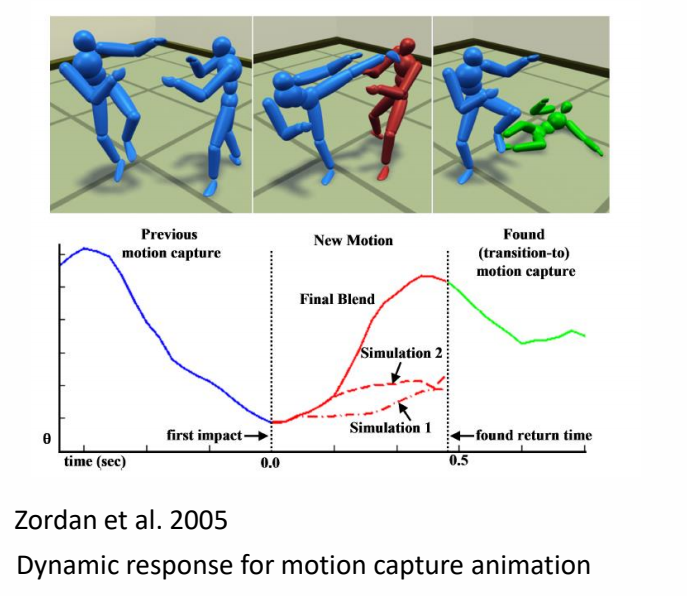
核心思想:关键帧与仿真的混合
- 用 mocap 提供目标轨迹
- 用仿真保证物理可行性
- 通过轨迹优化减小稳态误差
七、稳态误差 vs. 欠驱动问题
虽然两个问题都源于 PD 控制的局限性,但它们是不同的问题:
| 维度 | 稳态误差 | 欠驱动问题 |
|---|---|---|
| 本质 | 控制器设计问题 | 系统结构问题 |
| 原因 | 需要误差才能产生力矩 | 无法直接控制所有自由度 |
| 表现 | 动作滞后 | 质心不可控 |
| 解决 | 增大 \(k_p\)、前馈补偿 | 净外力、动量控制 |
| 是否可消除 | 可以(用前馈) | 不可以(系统特性) |
八、关键要点总结
-
稳态误差是 PD 控制的固有特性
- 需要误差才能产生力矩
- 有外力时必然存在稳态误差
-
在角色动画中的表现
- 动作滞后于参考轨迹
- Motion falls behind reference
-
解决方案
- 增大 \(k_p\):简单但有上限
- Stable PD:提高数值稳定性
- 前馈补偿:最有效,但需要模型
- PID:少用,可能振荡
-
与欠驱动问题的区别
- 稳态误差:控制器设计问题
- 欠驱动:系统结构问题
✅ 与前向/后向动力学的关系:
- 前向动力学:给定力求运动(仿真器)
- 后向动力学:给定运动求力(控制器)
- 稳态误差是后向动力学中的问题
📚 深入学习:
- Controlling Characters - PD 控制在角色上的应用
- 欠驱动系统问题 - PD 控制的另一个挑战
- 轨迹优化 - 通过优化目标轨迹来减小误差
本文出自 CaterpillarStudyGroup,转载请注明出处。 https://caterpillarstudygroup.github.io/GAMES105_mdbook/
前馈控制与反馈控制(Feedforward vs. Feedback Control)
✅ 本章定位:理解前馈控制和反馈控制的区别,以及 PD 控制在角色动画中的定位。
一、基本概念
反馈控制(Feedback Control)
定义:根据当前状态与目标状态的误差来调整控制输出。
$$ \tau = f(\text{当前状态}, \text{目标状态}) = f(e(t)) $$
核心特征:
- 依赖传感器测量当前状态
- 根据误差调整输出
- 可以抵抗扰动和不确定性
框图:
flowchart LR
    Ref[目标状态] --> Sum((+/-))
    Sum --> Controller[控制器]
    Controller --> Plant[被控对象]
    Plant --> Output[输出]
    Output --> Sensor[传感器]
    Sensor --> Sum
例子:
- PD 控制:\(\tau = k_p(q_{\text{des}} - q_{\text{curr}}) + k_d(\dot{q}{\text{des}} - \dot{q}{\text{curr}})\)
- 巡航控制:根据当前速度调整油门
- 恒温器:根据当前温度调整加热
前馈控制(Feedforward Control)
定义:根据目标状态和系统模型预先计算控制输出,不依赖当前状态测量。
$$ \tau = f(\text{目标状态}, \text{系统模型}) = f(q_{\text{des}}, M, C, G) $$
核心特征:
- 不依赖传感器
- 基于模型预先计算
- 无法抵抗未建模的扰动
框图:
flowchart LR
    Ref[目标状态] --> Controller[控制器]
    Controller --> Plant[被控对象]
    Plant --> Output[输出]
例子:
- 根据期望加速度预先计算需要的力矩
- 钢琴自动演奏:按预设程序执行
- 洗衣机:按预设程序运行,不检测衣服干净程度
二、核心区别
| 维度 | 反馈控制 | 前馈控制 |
|---|---|---|
| 输入 | 当前状态 + 目标状态 | 仅目标状态 + 模型 |
| 误差纠正 | ✅ 可以 | ❌ 不可以 |
| 抗扰动能力 | ✅ 强 | ❌ 弱 |
| 响应速度 | 受限于误差出现 | 可以预先动作 |
| 稳定性 | 可能振荡 | 取决于模型精度 |
| 模型依赖 | 低 | 高 |
三、PD 控制是反馈还是前馈?
这个问题很复杂...
从公式角度看:PD 是反馈控制
$$ \tau = k_p (q_{\text{des}} - q_{\text{curr}}) + k_d (\dot{q}{\text{des}} - \dot{q}{\text{curr}}) $$
反馈特征:
- 使用了当前状态 \(q_{\text{curr}}, \dot{q}_{\text{curr}}\)
- 根据误差 \(e = q_{\text{des}} - q_{\text{curr}}\) 计算输出
- 可以抵抗扰动
从系统角度看:PD 可以是前馈控制
在角色动画的完整系统中:
flowchart TB
    subgraph "中层策略"
        Traj[轨迹生成]
    end

    subgraph "底层执行"
        PD[PD 控制器]
    end

    subgraph "仿真器"
        Sim[物理仿真]
    end

    Traj -->|"目标状态 q*<br/>(位置,不是 q)"| PD
    PD -->|"力矩 τ"| Sim
    Sim -->|"新状态"| Traj
前馈特征:
- PD 的输入是轨迹生成器输出的 \(q^*\)
- \(q^*\) 是期望位置,不是当前状态 \(q\)
- PD 在这个层次上是执行器,不是控制器
正确答案:取决于观察层次
| 观察层次 | PD 控制类型 | 原因 |
|---|---|---|
| 关节级别 | 反馈控制 | 使用当前关节状态计算力矩 |
| 系统级别 | 前馈控制 | 目标状态由上层决定,PD 只是执行 |
四、PD 控制器的两种形式
1. 纯反馈 PD(无前馈项)
$$ \tau = k_p (q^* - q) + k_d (\dot{q}^* - \dot{q}) $$
| 特点 | 说明 |
|---|---|
| 力矩来源 | 100% 来自反馈项 |
| 输入 | 仅需目标状态 \((q^, \dot{q}^)\) |
| 优点 | 简单、无需轨迹优化 |
| 缺点 | 稳态误差大、响应滞后、需要较大增益 |
| 适用场景 | 简单动作、对精度要求不高 |
DeepMimic/AMP 等深度学习方法采用这种形式:
- RL 策略输出目标状态 \((q^, \dot{q}^)\)
- PD 控制器负责计算力矩
2. 前馈 - 反馈复合 PD(有前馈项)
$$ \tau = \underbrace{\tau^}_{\text{前馈}} + \underbrace{k_p (q^ - q) + k_d (\dot{q}^* - \dot{q})}_{\text{反馈}} $$
| 特点 | 说明 |
|---|---|
| 力矩来源 | 前馈 \(\tau^*\) + 反馈 \(\text{PD}\) |
| 输入 | 目标状态 \((q^, \dot{q}^)\) + 前馈力矩 \(\tau^*\) |
| 优点 | 跟踪精度高、稳态误差小、增益可设小、动作更自然 |
| 缺点 | 需要轨迹优化或逆动力学计算 \(\tau^*\) |
| 适用场景 | 高精度跟踪、复杂动作 |
前馈项 \(\tau^*\) 的来源:
- 轨迹优化:同时优化状态轨迹和控制轨迹,\(\tau^*\) 作为前馈项
- 逆动力学:给定期望运动 \((q^, \dot{q}^, \ddot{q}^*)\),计算需要的力矩
3. 两种形式的对比
| 维度 | 纯反馈 PD | 前馈 - 反馈复合 PD |
|---|---|---|
| 公式 | \(\tau = k_p e + k_d \dot{e}\) | \(\tau = \tau^* + k_p e + k_d \dot{e}\) |
| 力矩分配 | 反馈 100% | 前馈 60-80% + 反馈 20-40% |
| 跟踪精度 | 较低(有稳态误差) | 较高(前馈抵消大部分力) |
| 抗扰动能力 | 好 | 好 |
| 参数整定 | \(k_p, k_d\) 需较大 | \(k_p, k_d\) 可较小 |
| 动作自然度 | 可能僵硬 | 更自然流畅 |
| 计算成本 | 低 | 中(需计算 \(\tau^*\)) |
4. 直观类比:开车
| 纯反馈 PD | 前馈 - 反馈复合 PD | |
|---|---|---|
| 场景 | 新手开车上山 | 老司机开车上山 |
| 做法 | 看速度表,慢了加油,快了收油 | 凭经验预先加油门,同时微调 |
| 结果 | 能开,但速度波动大 | 开得平稳、省油 |
5. 实际建议
推荐方案:前馈 - 反馈复合控制
参数分配建议:
- 前馈项 \(\tau^*\):承担 60-80% 的跟踪任务
- 反馈项 \(k_p e + k_d \dot{e}\):承担 20-40% 的纠偏任务
好处:
- 反馈增益可以设小,动作更自然
- 前馈提供主要驱动力,跟踪更精确
- 反馈负责抗扰动,系统更鲁棒
五、在角色动画中的应用
纯反馈控制的局限
如果只用反馈控制:
$$ \tau = k_p (q_{\text{des}} - q_{\text{curr}}) + k_d (\dot{q}{\text{des}} - \dot{q}{\text{curr}}) $$
问题:
- 稳态误差:需要误差才能产生力矩
- 响应滞后:误差出现后才纠正
- 被动性:无法主动预测
前馈 + 反馈的组合控制
最优方案:结合前馈和反馈的优势
$$ \tau = \underbrace{k_p e + k_d \dot{e}}{\text{反馈}} + \underbrace{\tau{\text{feedforward}}}_{\text{前馈}} $$
其中前馈项:
$$ \tau_{\text{feedforward}} = M(q)\ddot{q}_{\text{des}} + C(q, \dot{q}) + G(q) $$
框图:
flowchart LR
    subgraph "前馈路径"
        Ref[目标状态] --> Model[逆动力学模型]
        Model --> Sum((+))
    end

    subgraph "反馈路径"
        Ref --> Sum2((+/-))
        Output[输出] --> Sensor[传感器]
        Sensor --> Sum2
        Sum2 --> PD[PD 控制器]
        PD --> Sum
    end

    Sum --> Plant[被控对象]
    Plant --> Output
优势:
- 前馈项负责精确跟踪目标
- 反馈项负责抵抗扰动
- 两者结合实现最优控制
六、DeepMimic/AMP 中的控制类型
DeepMimic 的控制架构
flowchart TB
    Mocap[参考动作] --> Reward[奖励函数]
    Reward --> RL[RL 策略训练]
    RL --> Policy[策略网络 π(a|s)]
    Policy --> PD[PD 控制器]
    PD --> Sim[物理仿真]
控制类型分析:
| 模块 | 控制类型 | 说明 |
|---|---|---|
| 策略网络 | 前馈 + 反馈 | 输入当前状态 s,输出动作 a |
| PD 控制器 | 反馈 | 使用当前关节状态计算力矩 |
| 整体系统 | 反馈 | 根据当前状态调整输出 |
AMP 的控制架构
flowchart LR
    Data[无标注 mocap] --> Discriminator[判别器 D]
    Discriminator --> Policy[策略π]
    Policy --> Sim[仿真]
    Sim --> Discriminator
控制类型:
- 对抗学习训练策略
- 策略输出关节力矩或 PD 目标
- 本质上是反馈控制
七、实际应用中的选择
何时使用反馈控制?
| 场景 | 原因 |
|---|---|
| 有外部扰动 | 反馈可以纠正误差 |
| 模型不确定 | 不依赖精确模型 |
| 需要鲁棒性 | 反馈提供稳定性 |
何时使用前馈控制?
| 场景 | 原因 |
|---|---|
| 已知轨迹 | 可以预先计算 |
| 快速响应 | 不需要等待误差 |
| 模型精确 | 前馈效果准确 |
最佳实践:组合使用
总控制 = 前馈(逆动力学) + 反馈(PD)
比例建议:
- 前馈:60-80%(承担主要跟踪任务)
- 反馈:20-40%(负责误差纠正)
八、关键要点总结
-
反馈控制
- 根据当前状态与目标的误差调整输出
- 可以抵抗扰动
- PD 控制是典型的反馈控制
-
前馈控制
- 根据目标状态和模型预先计算
- 无法抵抗未建模扰动
- 响应更快,可以"预见"动作
-
PD 控制的定位
- 关节级别:反馈控制
- 系统级别:前馈控制的执行器
- 完整系统:通常与前馈组合使用
-
实际应用
- 纯反馈:简单但有稳态误差
- 纯前馈:无法抵抗扰动
- 前馈 + 反馈:最优方案
九、与前向/后向动力学的关系
| 动力学类型 | 对应控制类型 | 说明 |
|---|---|---|
| 前向动力学 | - | 给定力求运动(仿真器) |
| 后向动力学 | 前馈控制 | 给定运动求力(逆动力学) |
关系:
- 前馈控制需要解决后向动力学问题
- 反馈控制只需要前向动力学(仿真)
📚 深入学习:
- 稳态误差问题 - 反馈控制的固有局限
- 欠驱动系统问题 - PD 控制的另一个挑战
- Controlling Characters - PD 控制在角色上的应用
- 轨迹优化 - 前馈控制的典型应用
本文出自 CaterpillarStudyGroup,转载请注明出处。 https://caterpillarstudygroup.github.io/GAMES105_mdbook/
P62
Static Balance
本章要解决的问题
核心问题:如何在静止站立的情况下,通过控制策略保证角色不摔倒?
问题分解
| 子问题 | 说明 |
|---|---|
| 什么是平衡? | 质心在支撑面内 |
| 为什么难? | 人形角色是欠驱动系统 |
| 如何检测不平衡? | 检查质心投影是否偏离支撑面中心 |
| 如何纠正? | 在关节上施加额外的力矩 |
与欠驱动系统的关系
欠驱动系统 → 无法直接控制质心 → 需要间接控制
                    ↓
        通过关节力矩控制质心位置
                    ↓
      在脚踝或髋关节施加额外力矩
两种控制策略
| 策略 | 方法 | 特点 |
|---|---|---|
| 简单 PD 控制 | 在脚踝/髋关节加额外力矩 | 简单直接,适用于静止站立 |
| Jacobian Transpose | 虚拟力 → 关节力矩转换 | 更灵活,可实现多种动作 |
✅ 深入学习:欠驱动系统问题 - 理解为什么质心无法直接控制
定义
What is balance?
✅ Static Balance:在不发生移动的情况下,通过简单的控制策略,保证角色不摔倒。 ✅ 平衡:质心在支撑面内。
P64
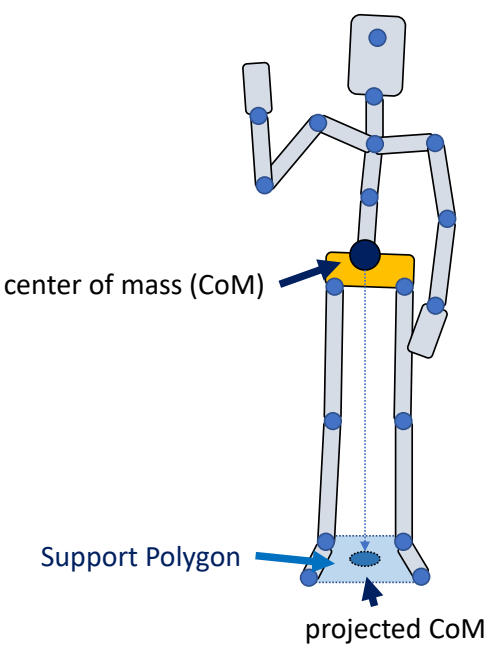
✅ 人的质心:每一段的质心的加权平均。
✅ 人的支撑面:两脚之内。
P66
A simple strategy: PD Control
A simple strategy to maintain balance:
根据条件计算力矩
-
Keep projected CoM close to the center of support polygon while tracking a standing pose
-
Use PD control to compute feedback torque
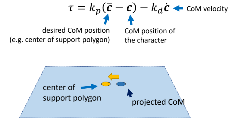
✅ 力矩 1:让角色保持某个姿势。
✅ 力矩 2:让质心与目标质心位置接近。力矩额外加在脚裸关节或髋关节上。
✅ 在某些关节上增加一些额外的力矩。
P68
施加力矩
- Apply the feedback torque at ankles (ankle strategy) or hips (hip strategy)
P69
Jacobian Transpose Control
✅ 实现 static balance,除了 PD 控制还有其它方法。
计算要施加的力
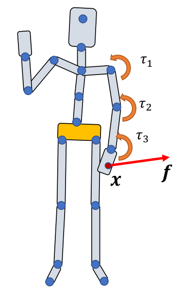
Can we use joint torques \(\tau _i\) to mimic the effect of a force \(f\) applied at \(x\)
- Note that the desired force \(f\) is not actually applied
- Also called “virtual force”
✅ 通过施加 \(\tau _1 ,\tau _2,\tau _3\) 来达到给 \(x\) 施加 \(f\) 的效果!
P73
把力转化为力矩
Make \(f\) and \(\tau _i\) done the same power
$$ P=f^T\dot{x}=\tau ^T\dot{\theta } $$
✅ 从做功的角度。力矩所做的功(功率)与虚力要做的功(功率)相同。功率 = \(fv\)
Forward kinematics \(x=g(\dot{\theta } )\Rightarrow \dot{x}=J \dot{\theta } \)
✅ \(g(* )\) 是一个FK函数。其中:
$$ J=\frac{\partial g}{\partial \theta } $$
✅ 把 \( \dot{x } \) 代入上面公式得
$$ f^T J\dot{\theta } = \tau ^T\dot{\theta } $$
$$ \Downarrow $$
P76
$$ \tau =J^Tf $$
✅ 把 \( \tau\) 分解为每一个关节每一个旋转的 \( \tau\).通过 Jacobian 矩阵的含义推出:
$$ \Downarrow $$
$$ \tau _i=(x-p_i)\times f $$
P77
用于Static Balance
A simple strategy to maintain balance:
-
Keep projected CoM close to the center of support polygon while tracking a standing pose
-
Use PD control to compute feedback virtual force
✅ P66 中在 Hips 上加力矩的方式只能进行简单的控制。
✅ 可以通过虚力实现相似的效果。用 \(PD\) 控制计算出力,再通过关节力矩实现这个力。
$$ f=k_p(\bar{c} -c)-k_d\dot{c} $$
✅ \(c\) 不一定是投影距离,还可以描述高度距离,实现站起蹲下的效果。
P78
- Assuming \(f\) is applied to the CoM, compute necessary joint torques using Jacobian transpose control to achieve it
✅ 但也不是真的加力,而是通过前面讲的 Jacobian transpose control 方法转为特定关节的力矩。
- Usually using the joints in the legs
✅ 最后达到在Hips上加力的效果
✅ 但这种方式能施加的力非常弱,只能实现比较微弱的平衡
P79
A fancier strategy:
- Mocap tracking as an objective function
- Controlling both the CoM position/momentum and the angular momentum
- Solve a one-step optimization problem to compute joint torques
🔎
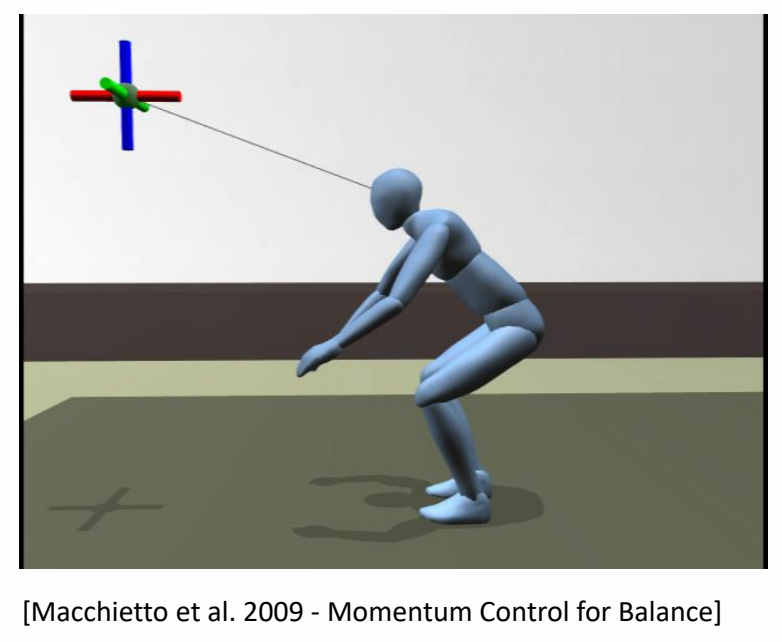
本文出自 CaterpillarStudyGroup,转载请注明出处。 https://caterpillarstudygroup.github.io/GAMES105_mdbook/
轨迹优化
✅ 本章定位:理解如何通过优化方法生成物理可行的目标轨迹,供 PD 控制器跟踪。
在控制系统中的位置
flowchart TD
    subgraph "高层:任务规划"
        A["做什么动作?<br/>有限状态机、行为树"]
    end

    subgraph "中层:轨迹生成 (本章)"
        B["如何生成目标动作?<br/>轨迹优化、DeepMimic、AMP"]
    end

    subgraph "底层:执行控制"
        C["如何计算关节力矩?<br/>PD 控制"]
    end

    subgraph "仿真器"
        D["物理仿真<br/>Mv̇ + C = f + Jᵀλ"]
    end

    A -->|动作指令 | B
    B -->|目标状态 q*, q̇* | C
    C -->|关节力矩 τ | D
    D -->|当前状态 q, q̇ | C
轨迹优化的输入输出:
- 输入:参考轨迹 ((q^{\text{ref}}, \dot{q}^{\text{ref}})) + (可选)当前状态
- 输出:目标轨迹 ((q^, \dot{q}^)) + 控制轨迹 ((\tau^*)) → 送入 PD 控制器
与 PD 控制的关系:
- 轨迹优化输出目标轨迹 ((q^, \dot{q}^)) → PD 控制的目标
- 轨迹优化输出控制轨迹 ((\tau^*)) → PD 控制的前馈项
- PD 控制计算力矩:(\tau = \tau^* + k_p(q^* - q) + k_d(\dot{q}^* - \dot{q}))
轨迹优化的输入来源
轨迹优化需要参考轨迹作为输入,参考轨迹主要有三类来源:
| 输入来源 | 说明 | 特点 |
|---|---|---|
| 动作捕捉(Mocap) | 从真实演员捕捉的运动数据 | 真实自然,但可能物理不可行 |
| 运动学方法生成 | Motion Matching、PFNN、扩散模型等 | 数据驱动、实时生成,但无物理约束 |
| 动画师制作 | 手工关键帧动画 | 艺术可控,但耗时、可能不符合物理 |
轨迹优化的作用:
- 对上述输入进行物理修正
- 使其满足动力学约束(运动方程、接触约束等)
- 输出物理可行的目标轨迹供 PD 控制跟踪
flowchart LR
    Input["输入:<br/>Mocap / 运动学方法 / 关键帧"] --> Opt["轨迹优化<br/>(物理修正)"]
    Opt --> PD["PD 控制"]
    PD --> Sim["物理仿真"]
✅ 本章聚焦轨迹优化:理解如何通过优化方法对参考轨迹进行物理修正。
四种轨迹的关系
轨迹优化涉及四种轨迹,它们的关系如下:
| 概念 | 符号 | 是什么 | 优化前/后 | 角色 |
|---|---|---|---|---|
| 参考轨迹 | ((q^{\text{ref}}, \dot{q}^{\text{ref}})) | 动捕/运动学方法/动画师提供的原始轨迹 | 优化前 | 轨迹优化的输入 |
| 状态轨迹 | ((q, \dot{q})) | 角色在每一帧的实际状态(位置 + 速度) | 通用术语 | 可指任何轨迹 |
| 目标轨迹 | ((q^, \dot{q}^)) | 轨迹优化后得到的物理可行轨迹 | 优化后 | 轨迹优化的输出 → PD 控制的目标 |
| 控制轨迹 | ((\tau)) | 每一帧的关节力矩序列 | 优化后 | 轨迹优化的输出 → PD 控制的前馈项 |
完整流程
参考轨迹 (q^ref, q̇^ref)  ← 来自动捕/运动学方法/动画师
    ↓
轨迹优化(物理修正)
    ↓
    ├──→ 目标轨迹 (q*, q̇*)  → 送给 PD 控制器作为目标
    └──→ 控制轨迹 (τ*)      → 送给 PD 控制器作为前馈项
关键对比
| 参考轨迹 | 目标轨迹 | 控制轨迹 | |
|---|---|---|---|
| 是什么 | "期望的动作" | "修正后的可行动作" | "产生动作需要的力" |
| 物理可行性 | ❌ 可能不可行 | ✅ 可行 | ✅ 可行 |
| 送给谁 | 轨迹优化 | PD 控制器 | PD 控制器(前馈) |
| 类比 | 设计师的设计图 | 工程师的施工图 | 施工用的材料清单 |
为什么需要轨迹优化
直接用 PD 控制跟踪动捕数据会有很大问题:
| 问题 | 原因 | 表现 |
|---|---|---|
| 稳态误差 | PD 控制需要误差才能产生力矩 | 动作滞后于参考轨迹 |
| 相位漂移 | 运动轨迹与原轨迹之间存在相位差 | 动作节奏不匹配 |
| 欠驱动问题 | 人形角色缺少对根节点的直接控制 | 质心位置无法直接控制 |
✅ 深入学习:欠驱动系统问题 - 详细讲解欠驱动系统的挑战和解决方案。
轨迹优化的作用:
- 在 mocap 基础上添加修正量,使其物理可行
- 引入轨迹优化之后,控制本质上变成了设计 target state
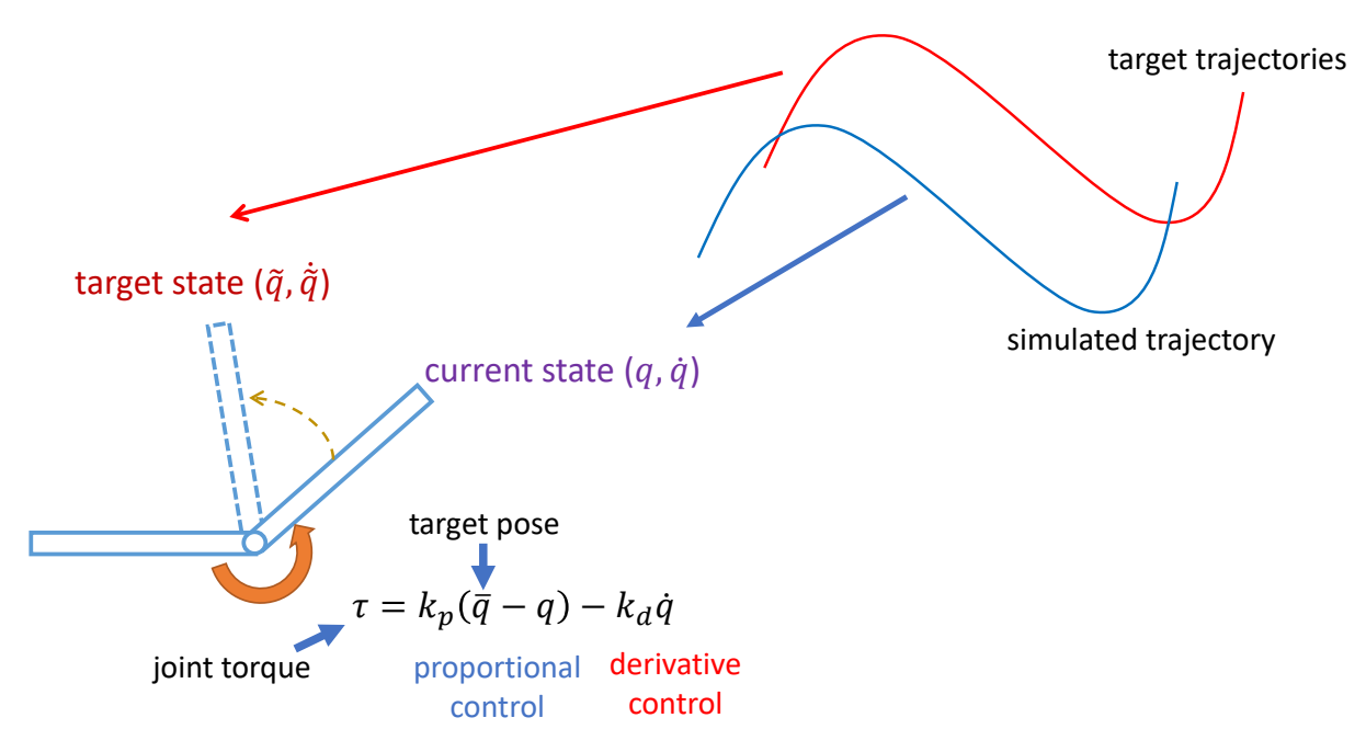
📖 数学形式化描述:详见 数学形式化描述 - 轨迹优化问题的完整数学描述。
本文出自 CaterpillarStudyGroup,转载请注明出处。 https://caterpillarstudygroup.github.io/GAMES105_mdbook/
轨迹优化的数学描述
✅ 本章定位:理解轨迹优化问题的数学形式化描述,包括优化变量、目标函数、约束条件。
一、问题概述
轨迹优化(Trajectory Optimization)的目标是:
找到一条状态轨迹和控制轨迹,使得在满足所有约束的前提下,最小化目标函数。
二、优化变量
状态轨迹(State Trajectory)
$$ \mathbf{x} _{0:T} = (\mathbf{x} _0, \mathbf{x} _1, \dots, \mathbf{x} _T) $$
其中每个状态 \(\mathbf{x} _t\) 包含:
| 变量 | 符号 | 维度 | 说明 |
|---|---|---|---|
| 位置 | \(\mathbf{q}\) | \(n\) | 关节角度 + 根节点位置 |
| 速度 | \(\dot{\mathbf{q}}\) | \(n\) | 关节角速度 + 根节点速度 |
对于人形角色,通常 \(n \approx 34\)(3DOF 根节点 + 31DOF 关节)。
控制轨迹(Control Trajectory)
$$ \mathbf{u} _{0:T-1} = (\mathbf{u} _0, \mathbf{u} _1, \dots, \mathbf{u} _{T-1}) $$
其中每个控制 \(\mathbf{u} _t\) 包含:
| 变量 | 符号 | 维度 | 说明 |
|---|---|---|---|
| 关节力矩 | \(\boldsymbol{\tau}\) | \(n _{\text{joint}}\) | 每个关节的力矩 |
| 根节点力 | \(\mathbf{f} _{\text{root}}\) | 3 | 虚拟外力(可选) |
| 根节点力矩 | \(\boldsymbol{\tau} _{\text{root}}\) | 3 | 虚拟外力矩(可选) |
三、目标函数
一般形式
$$ \min _{\mathbf{x} _{0:T}, \mathbf{u} _{0:T-1}} J(\mathbf{x} _{0:T}, \mathbf{u} _{0:T-1}) = J _T(\mathbf{x} _T) + \sum _{t=0} ^{T-1} J _t(\mathbf{x} _t, \mathbf{u} _t) $$
| 项 | 名称 | 说明 |
|---|---|---|
| \(J _T(\mathbf{x} _T)\) | 终端代价(Terminal Cost) | 关于终点状态的代价 |
| \(J _t(\mathbf{x} _t, \mathbf{u} _t)\) | 运行代价(Running Cost) | 关于每步状态和控制的代价 |
常见的运行代价项
1. 跟踪误差(Tracking Error)
$$ J _{\text{track}} = \sum _{t=0} ^{T-1} |\mathbf{q} _t - \mathbf{q} _t^{\text{ref}}|^2 $$
- \(\mathbf{q} _t^{\text{ref}}\):参考轨迹(来自动捕等)
- 作用:让优化结果贴近参考动作
2. 控制 Effort
$$ J _{\text{control}} = \sum _{t=0} ^{T-1} |\boldsymbol{\tau} _t|^2 $$
- 作用:最小化关节力矩,使动作更节能、更平滑
3. 速度平滑项
$$ J _{\text{smooth}} = \sum _{t=0} ^{T-1} |\dot{\mathbf{q}} _{t+1} - \dot{\mathbf{q}} _t|^2 $$
- 作用:减少速度突变,使动作更流畅
4. 质心高度项
$$ J _{\text{com}} = \sum _{t=0} ^{T-1} (h _{\text{com},t} - h _{\text{com}}^{\text{ref}})^2 $$
- 作用:维持质心高度,防止摔倒
完整的运行代价
$$ \begin{aligned} J _t(\mathbf{x} _t, \mathbf{u} _t) = ;&w _{\text{track}} |\mathbf{q} _t - \mathbf{q} _t^{\text{ref}}|^2 \\ &+ w _{\text{control}} |\boldsymbol{\tau} _t|^2 \\ &+ w _{\text{smooth}} |\dot{\mathbf{q}} _{t+1} - \dot{\mathbf{q}} _t|^2 \\ &+ w _{\text{com}} (h _{\text{com},t} - h _{\text{com}}^{\text{ref}})^2 \end{aligned} $$
其中 \(w_i\) 是权重系数,用于调节各项的重要性。
常见的终端代价
$$ J _T(\mathbf{x} _T) = w _{\text{vel}} |\dot{\mathbf{q}} _T|^2 + w _{\text{com}} (h _{\text{com},T} - h _{\text{com}}^{\text{ref}})^2 $$
- \(|\dot{\mathbf{q}}_T|^2\):终点速度为零(确保静止)
- \(h_{\text{com},T}\):终点质心高度(确保平衡)
四、约束条件
1. 动力学约束(Dynamics Constraint)
$$ M(\mathbf{q} _t)\ddot{\mathbf{q}} _t + C(\mathbf{q} _t, \dot{\mathbf{q}} _t) = \boldsymbol{\tau} _t + \mathbf{J}(\mathbf{q} _t)^T \boldsymbol{\lambda} _t $$
| 符号 | 说明 |
|---|---|
| \(M(\mathbf{q})\) | 质量矩阵 |
| \(C(\mathbf{q}, \dot{\mathbf{q}})\) | 科里奥利力 + 离心力 + 重力 |
| \(\boldsymbol{\tau}\) | 关节力矩(控制输入) |
| \(\mathbf{J}^T \boldsymbol{\lambda}\) | 约束力(接触力等) |
2. 运动学约束(Kinematic Constraint)
$$ \mathbf{g}(\mathbf{q} _t) = 0 $$
例如:
- 末端执行器位置约束
- 关节角度限制
3. 接触约束(Contact Constraint)
不穿透约束
$$ \phi(\mathbf{q} _t) \geq 0 $$
- \(\phi(\mathbf{q})\):接触点到地面的距离
- \(\phi > 0\):在空中
- \(\phi = 0\):接触地面
摩擦力约束(摩擦锥)
$$ |\mathbf{f} _{\text{tangential}}| \leq \mu \cdot f _{\text{normal}} $$
- \(\mu\):摩擦系数
- 防止脚在地面上滑动
4. 控制约束(Control Constraint)
$$ \boldsymbol{\tau} _{\min} \leq \boldsymbol{\tau} _t \leq \boldsymbol{\tau} _{\max} $$
- 关节力矩有物理上限
5. 状态约束(State Constraint)
$$ \mathbf{q} _{\min} \leq \mathbf{q} _t \leq \mathbf{q} _{\max} $$
$$ \dot{\mathbf{q}} _{\min} \leq \dot{\mathbf{q}} _t \leq \dot{\mathbf{q}} _{\max} $$
- 关节角度限制(生理范围)
- 速度限制
五、完整的优化问题
$$ \begin{aligned} \min _{\mathbf{x} _{0:T}, \mathbf{u} _{0:T-1}} \quad & J _T(\mathbf{x} _T) + \sum _{t=0} ^{T-1} J _t(\mathbf{x} _t, \mathbf{u} _t) \\ \text{s.t.} \quad & M(\mathbf{q} _t)\ddot{\mathbf{q}} _t + C(\mathbf{q} _t, \dot{\mathbf{q}} _t) = \boldsymbol{\tau} _t + \mathbf{J}(\mathbf{q} _t)^T \boldsymbol{\lambda} _t & \text{(动力学)} \\ & \phi(\mathbf{q} _t) \geq 0 & \text{(不穿透)} \\ & |\mathbf{f} _{\text{tangential}}| \leq \mu \cdot f _{\text{normal}} & \text{(摩擦锥)} \\ & \boldsymbol{\tau} _{\min} \leq \boldsymbol{\tau} _t \leq \boldsymbol{\tau} _{\max} & \text{(控制限制)} \\ & \mathbf{q} _{\min} \leq \mathbf{q} _t \leq \mathbf{q} _{\max} & \text{(状态限制)} \end{aligned} $$
六、问题建模
对这个问题用不同的方式建模,会得到不同的方法:
| 动态规划问题 | Find a path {\(s _t\)} that minimizes | \(J(s _0)=\sum _ {t=0}^{ } h(s _t,s _{t+1})\) |
| 轨迹问题 | Find a sequence of action {\(a _t\)} that minimizes | \(J(s _0)=\sum _ {t=0}^{ } h(s _t,a _t)\) subject to \( s _{t+1}=f(s _t,a _t)\) |
| 控制策略问题 | Find a policy \( a _t=\pi (s _t,t)\)或 \( a _t=\pi (s _t)\)that minimizes | \(J(s _0)=\sum _ {t=0}^{ } h(s _t,a _t)\) subject to \(s _{t+1}=f(s _t,a _t)\) |
六、关键要点总结
-
优化变量:状态轨迹 \(\mathbf{x} _{0:T}\) + 控制轨迹 \(\mathbf{u} _{0:T-1}\)
-
目标函数:
- 终端代价 \(J _T(\mathbf{x} _T)\)
- 运行代价 \(\sum J _t(\mathbf{x} _t, \mathbf{u} _t)\)
- 常见项:跟踪误差、控制 effort、平滑项
-
约束条件:
- 动力学约束(运动方程)
- 接触约束(不穿透、摩擦锥)
- 控制/状态限制
📚 深入学习:
本文出自 CaterpillarStudyGroup,转载请注明出处。 https://caterpillarstudygroup.github.io/GAMES105_mdbook/
轨迹优化相关概念澄清
✅ 本章定位:澄清轨迹优化中容易混淆的概念,包括离线/在线、开环/闭环、前馈/反馈三组概念的区别与联系。
三组容易混淆的概念
轨迹优化领域有三组分类概念,它们经常被混用,但实际上是三个不同维度的分类:
| 维度 | 分类 | 核心问题 |
|---|---|---|
| 维度 1:优化时机 | 离线 vs. 在线 | 什么时候计算控制策略? |
| 维度 2:控制方式 | 开环 vs. 闭环 | 是否使用当前状态反馈? |
| 维度 3:力矩来源 | 前馈 vs. 反馈 | 力矩从哪里来? |
维度 1:离线优化 vs. 在线优化(Optimization Timing)
定义
| 离线优化 | 在线优化 | |
|---|---|---|
| 计算时机 | 任务执行前预先计算 | 任务执行中实时计算 |
| 计算频率 | 一次(或偶尔重新计算) | 每帧/每隔几帧 |
| 输出 | 完整的轨迹/策略 | 当前步的轨迹/策略 |
| 计算时间 | 可以很长(秒/分钟级) | 必须很短(毫秒级) |
代表方法
| 离线优化 | 在线优化 | |
|---|---|---|
| 轨迹优化 | CMA-ES、iLQR、DDP | MPC、SAMCON |
| 学习方法 | DeepMimic(训练阶段) | DeepMimic(推理阶段) |
优缺点对比
| 维度 | 离线优化 | 在线优化 |
|---|---|---|
| 计算成本 | 低(只做一次) | 高(持续计算) |
| 抗扰动能力 | ❌ 弱(无法应对意外) | ✅ 强(可实时调整) |
| 适用场景 | 预先制作动作库 | 实时交互控制 |
直观类比
| 离线优化 | 在线优化 | |
|---|---|---|
| 开车 | 出门前查好导航路线 | 根据实时路况调整路线 |
| 做饭 | 按菜谱步骤执行 | 根据食材状态调整火候 |
| 结果 | 路线最优但怕堵车 | 可避开拥堵但计算成本高 |
维度 2:开环控制 vs. 闭环控制(Control Architecture)
定义
| 开环控制 | 闭环控制 | |
|---|---|---|
| 是否使用反馈 | ❌ 不使用当前状态 | ✅ 使用当前状态 |
| 输入 | 仅初始状态 + 预设指令 | 初始状态 + 实时状态反馈 |
| 抗扰动能力 | ❌ 弱(扰动后无法恢复) | ✅ 强(可纠正偏差) |
| 输出 | 预设动作序列 | 根据状态调整的动作 |
框图对比
开环控制:
初始状态 → 控制器 → 动作序列 → 执行 → 结果
闭环控制:
              ┌──────────────┐
              │              │
              ▼              │
目标状态 → (+) → 控制器 → 执行 → 当前状态
              ▲              │
              │              │
              └─────传感器───┘
                (状态反馈)
代表方法
| 开环控制 | 闭环控制 | |
|---|---|---|
| 轨迹跟踪 | 纯轨迹跟踪(无 PD) | PD 跟踪、MPC |
| 特点 | 简单但脆弱 | 鲁棒但复杂 |
优缺点对比
| 维度 | 开环控制 | 闭环控制 |
|---|---|---|
| 结构简单 | ✅ 简单 | ❌ 需要传感器/反馈 |
| 抗扰动 | ❌ 无 | ✅ 强 |
| 精度 | ❌ 依赖模型精度 | ✅ 可纠正误差 |
| 稳定性 | ❌ 可能发散 | ✅ 通常稳定 |
直观类比
| 开环控制 | 闭环控制 | |
|---|---|---|
| 投篮 | 闭眼投出,不调整 | 看着篮筐,实时调整 |
| 开车 | 闭眼开,只靠预设方向盘 | 看着路,随时修正方向 |
| 结果 | 有扰动就偏离 | 可抵抗扰动 |
维度 3:前馈控制 vs. 反馈控制(Torque Source)
定义
| 前馈控制 | 反馈控制 | |
|---|---|---|
| 力矩来源 | 预先计算的力矩 $\tau^*$ | 根据误差计算的力矩 |
| 计算公式 | $\tau = f(\text{模型}, \text{目标})$ | $\tau = k_p e + k_d \dot{e}$ |
| 是否需要模型 | ✅ 需要(逆动力学) | ⚠️ 需要较少 |
| 响应速度 | 快(无需等待误差) | 慢(需要误差出现) |
公式对比
前馈控制: $$ \tau_{\text{feedforward}} = \text{InverseDynamics}(q^, \dot{q}^, \ddot{q}^*) $$
反馈控制(PD): $$ \tau_{\text{feedback}} = k_p (q^* - q) + k_d (\dot{q}^* - \dot{q}) $$
复合控制(前馈 + 反馈): $$ \tau = \underbrace{\tau_{\text{feedforward}}}{\text{前馈}} + \underbrace{k_p (q^* - q) + k_d (\dot{q}^* - \dot{q})}{\text{反馈}} $$
代表方法
| 前馈控制 | 反馈控制 | |
|---|---|---|
| 方法 | 轨迹优化的控制轨迹、逆动力学 | PD 控制、 Stable PD |
| 特点 | 精确但需要模型 | 鲁棒但有稳态误差 |
优缺点对比
| 维度 | 前馈控制 | 反馈控制 |
|---|---|---|
| 响应速度 | ✅ 快(预先计算) | ❌ 慢(需误差出现) |
| 模型依赖 | ❌ 高(需要精确模型) | ✅ 低 |
| 抗扰动 | ❌ 弱 | ✅ 强 |
| 稳态误差 | ✅ 无 | ❌ 有(需要误差才能输出力矩) |
直观类比
| 前馈控制 | 反馈控制 | |
|---|---|---|
| 弹琴 | 记住谱子,凭肌肉记忆弹奏 | 听音准,实时调整手指 |
| 开车上山 | 凭经验预先踩油门 | 看速度表,慢了加油快了收油 |
| 最佳方案 | 记住谱子 + 听音调整(前馈 + 反馈) |
三组概念的关系
核心区别
| 概念对 | 核心问题 | 与其他概念的关系 |
|---|---|---|
| 离线 vs. 在线 | 什么时候计算? | 决定前馈力矩的计算时机 |
| 开环 vs. 闭环 | 是否用反馈? | 闭环 = 有反馈控制 |
| 前馈 vs. 反馈 | 力矩从哪里来? | 前馈通常来自离线/在线优化 |
常见组合方案
方案 1:离线优化 + 前馈 + 反馈(最常用)
离线轨迹优化 → 目标轨迹 (q*, q̇*) + 控制轨迹 (τ*)
                        ↓
              在线 PD 控制:τ = τ* + k_p·e + k_d·ė
                        ↓
              闭环控制(前馈 + 反馈)
| 维度 | 选择 | 说明 |
|---|---|---|
| 优化时机 | 离线 | 预先计算轨迹和控制 |
| 控制方式 | 闭环 | 使用 PD 反馈 |
| 力矩来源 | 前馈 + 反馈 | $\tau = \tau^* + \text{PD}$ |
优点:
- 前馈提供主要驱动力(60-80%)
- 反馈负责抗扰动和纠偏(20-40%)
- 计算成本低(离线优化一次)
适用场景:动捕跟踪、预先制作的动作
方案 2:在线优化 + 前馈 + 反馈(MPC)
每帧:
  1. 测量当前状态 x
  2. 在线优化 → 新目标轨迹 + 新控制轨迹 (τ*)
  3. PD 控制:τ = τ* + k_p·e + k_d·ė
| 维度 | 选择 | 说明 |
|---|---|---|
| 优化时机 | 在线 | 每帧重新优化 |
| 控制方式 | 闭环 | 使用当前状态反馈 |
| 力矩来源 | 前馈 + 反馈 | $\tau = \tau^* + \text{PD}$ |
优点:
- 可应对动态变化的环境
- 可处理突发扰动
缺点:
- 计算成本高
- 需要高效求解器
适用场景:实时交互、复杂地形行走
方案 3:纯反馈(DeepMimic)
RL 策略 → 目标轨迹 (q*, q̇*)
              ↓
PD 控制:τ = k_p·e + k_d·ė(无前馈)
| 维度 | 选择 | 说明 |
|---|---|---|
| 优化时机 | 离线(训练) | 训练一次,推理多次 |
| 控制方式 | 闭环 | 使用 PD 反馈 |
| 力矩来源 | 纯反馈 | $\tau = \text{PD}$ only |
优点:
- 无需轨迹优化
- 策略可泛化
缺点:
- 需要大量训练
- 稳态误差较大
适用场景:通用角色控制、游戏 AI
完整对比表
| 方案 | 优化时机 | 控制方式 | 力矩来源 | 抗扰动 | 计算成本 | 代表方法 |
|---|---|---|---|---|---|---|
| 方案 1 | 离线 | 闭环 | 前馈 + 反馈 | ✅ | 低 | 轨迹优化 + PD |
| 方案 2 | 在线 | 闭环 | 前馈 + 反馈 | ✅✅ | 高 | MPC |
| 方案 3 | 离线 | 闭环 | 纯反馈 | ✅ | 中 | DeepMimic |
| 方案 4 | 离线 | 开环 | 纯前馈 | ❌ | 最低 | 纯轨迹跟踪 |
关键要点总结
-
三组概念是不同维度的分类
- 离线/在线:什么时候计算
- 开环/闭环:是否用反馈
- 前馈/反馈:力矩从哪里来
-
常见组合方案
- 最佳实践:离线优化 + 闭环控制 + 前馈 + 反馈
- 实时应用:在线优化(MPC)+ 闭环控制
- 学习方法:离线训练 + 闭环控制 + 纯反馈
-
概念关系
- 离线/在线优化 → 输出前馈力矩
- 开环/闭环 → 决定是否使用反馈
- 前馈/反馈 → 力矩的两个来源,可以组合使用
-
选择建议
- 需要抗扰动 → 闭环 + 反馈
- 需要精确跟踪 → 加前馈
- 计算资源有限 → 离线优化
- 环境动态变化 → 在线优化(MPC)
📚 深入学习:
本文出自 CaterpillarStudyGroup,转载请注明出处。 https://caterpillarstudygroup.github.io/GAMES105_mdbook/
轨迹优化方法对比与分类
✅ 本章定位:全面梳理轨迹优化领域的知识体系,通过多维度分类、方法对比和关系图谱,建立对各种优化方法的整体认知。
⭐ 重要概念区分:框架 vs. 求解器
在轨迹优化领域,需要区分控制框架和具体求解器:
| 控制框架 | 具体求解器 | |
|---|---|---|
| 定义 | 定义"何时优化、如何执行"的控制范式 | 实际求解优化问题的算法 |
| 代表 | MPC(模型预测控制) | LQR、iLQR、DDP、CMA-ES、SAMCON |
| 关系 | 框架可以结合不同的求解器 | 求解器可以服务于不同的框架 |
| 类比 | 汽车的"自动驾驶系统" | 汽车的"发动机"(汽油/柴油/电动) |
MPC 框架 + 不同求解器
MPC 框架(滚动时域优化)
    │
    ├─ 结合 LQR 求解器     →  LQR-MPC(仅限线性系统)
    │
    ├─ 结合 iLQR 求解器    →  iLQR-MPC(适用于平滑非线性问题)⭐最常用
    │
    ├─ 结合 DDP 求解器     →  DDP-MPC(适用于高精度需求)
    │
    ├─ 结合 CMA-ES        →  Sampling-MPC(适用于不可微问题)
    │
    ├─ 结合 SAMCON        →  粒子滤波 MPC(适用于角色控制)
    │
    └─ 结合凸优化         →  Convex-MPC(适用于凸问题)
关键理解:
- MPC 不是算法,是框架 —— 它定义了"每帧优化、只执行第一步"的思想
- 求解器是具体实现 —— 它实际计算最优控制序列
- 同一个 MPC 框架,换不同求解器,适用于不同问题
一、方法全景图(Mind Map)
mindmap
  root((轨迹优化方法))
    按优化时机
      离线优化
        CMA-ES
        iLQR
        DDP
        :: icon(fa fa-clock-o)
        一次性计算
        适用于动作生成
      在线优化
        MPC
        SAMCON
        :: icon(fa fa-refresh)
        每帧重新计算
        适用于实时控制
    按求解方法
      解析法
        LQR
        :: icon(fa fa-check)
        闭式解
        仅限线性系统
      数值法
        基于梯度
          iLQR 一阶
          DDP 二阶
        无梯度
          CMA-ES
          SAMCON
      学习法
        DeepMimic
        AMP
        :: icon(fa fa-brain)
        训练一次推理多次
    按控制方式
      开环控制
        纯轨迹跟踪
        :: icon(fa fa-chain)
        无反馈
      闭环控制
        PD 控制
        MPC
        :: icon(fa fa-sync)
        状态反馈
    按力矩来源
      前馈控制
        逆动力学
        轨迹优化输出
        :: icon(fa fa-forward)
      反馈控制
        PD 控制
        :: icon(fa fa-undo)
      复合控制
        前馈 + 反馈
        :: icon(fa fa-plus)
    典型应用场景
      动作生成
        iLQR DDP CMA-ES
      实时控制
        MPC SAMCON
      通用策略
        DeepMimic AMP
二、三组核心分类概念
轨迹优化领域有三组分类概念,它们经常被混用,但实际上是三个不同维度的分类:
| 维度 | 分类 | 核心问题 |
|---|---|---|
| 维度 1:优化时机 | 离线 vs. 在线 | 什么时候计算控制策略? |
| 维度 2:控制方式 | 开环 vs. 闭环 | 是否使用当前状态反馈? |
| 维度 3:力矩来源 | 前馈 vs. 反馈 | 力矩从哪里来? |
维度 1:离线优化 vs. 在线优化(Optimization Timing)
| 离线优化 | 在线优化 | |
|---|---|---|
| 计算时机 | 任务执行前预先计算 | 任务执行中实时计算 |
| 计算频率 | 一次(或偶尔重新计算) | 每帧/每隔几帧 |
| 输出 | 完整的轨迹/策略 | 当前步的轨迹/策略 |
| 计算时间 | 可以很长(秒/分钟级) | 必须很短(毫秒级) |
代表方法:
| 离线优化 | 在线优化 | |
|---|---|---|
| 轨迹优化 | CMA-ES、iLQR、DDP | MPC、SAMCON |
| 学习方法 | DeepMimic(训练阶段) | DeepMimic(推理阶段) |
优缺点对比:
| 维度 | 离线优化 | 在线优化 |
|---|---|---|
| 计算成本 | 低(只做一次) | 高(持续计算) |
| 抗扰动能力 | ❌ 弱(无法应对意外) | ✅ 强(可实时调整) |
| 适用场景 | 预先制作动作库 | 实时交互控制 |
直观类比:
| 离线优化 | 在线优化 | |
|---|---|---|
| 开车 | 出门前查好导航路线 | 根据实时路况调整路线 |
| 做饭 | 按菜谱步骤执行 | 根据食材状态调整火候 |
维度 2:开环控制 vs. 闭环控制(Control Architecture)
| 开环控制 | 闭环控制 | |
|---|---|---|
| 是否使用反馈 | ❌ 不使用当前状态 | ✅ 使用当前状态 |
| 输入 | 仅初始状态 + 预设指令 | 初始状态 + 实时状态反馈 |
| 抗扰动能力 | ❌ 弱(扰动后无法恢复) | ✅ 强(可纠正偏差) |
| 输出 | 预设动作序列 | 根据状态调整的动作 |
框图对比:
开环控制:
初始状态 → 控制器 → 动作序列 → 执行 → 结果
闭环控制:
              ┌──────────────┐
              │              │
              ▼              │
目标状态 → (+) → 控制器 → 执行 → 当前状态
              ▲              │
              │              │
              └─────传感器───┘
                (状态反馈)
优缺点对比:
| 维度 | 开环控制 | 闭环控制 |
|---|---|---|
| 结构简单 | ✅ 简单 | ❌ 需要传感器/反馈 |
| 抗扰动 | ❌ 无 | ✅ 强 |
| 精度 | ❌ 依赖模型精度 | ✅ 可纠正误差 |
| 稳定性 | ❌ 可能发散 | ✅ 通常稳定 |
维度 3:前馈控制 vs. 反馈控制(Torque Source)
| 前馈控制 | 反馈控制 | |
|---|---|---|
| 力矩来源 | 预先计算的力矩 $\tau^*$ | 根据误差计算的力矩 |
| 计算公式 | $\tau = f(\text{模型}, \text{目标})$ | $\tau = k_p e + k_d \dot{e}$ |
| 是否需要模型 | ✅ 需要(逆动力学) | ⚠️ 需要较少 |
| 响应速度 | 快(无需等待误差) | 慢(需要误差出现) |
公式对比:
前馈控制: $$ \tau_{\text{feedforward}} = \text{InverseDynamics}(q^, \dot{q}^, \ddot{q}^*) $$
反馈控制(PD): $$ \tau_{\text{feedback}} = k_p (q^* - q) + k_d (\dot{q}^* - \dot{q}) $$
复合控制(前馈 + 反馈): $$ \tau = \underbrace{\tau_{\text{feedforward}}}{\text{前馈}} + \underbrace{k_p (q^* - q) + k_d (\dot{q}^* - \dot{q})}{\text{反馈}} $$
优缺点对比:
| 维度 | 前馈控制 | 反馈控制 |
|---|---|---|
| 响应速度 | ✅ 快(预先计算) | ❌ 慢(需误差出现) |
| 模型依赖 | ❌ 高(需要精确模型) | ✅ 低 |
| 抗扰动 | ❌ 弱 | ✅ 强 |
| 稳态误差 | ✅ 无 | ❌ 有(需要误差才能输出力矩) |
四、四种维度分类法
轨迹优化方法可以从四个维度进行分类:
维度 1:按优化时机(输入信息)
| 离线优化 | 在线优化 | |
|---|---|---|
| 输入 | 仅参考轨迹 | 参考轨迹 + 当前状态 |
| 优化频率 | 一次(整条轨迹) | 每帧/实时(滚动优化) |
| 代表方法 | CMA-ES、iLQR、DDP、DeepMimic(训练) | MPC、SAMCON、DeepMimic(推理) |
| 优点 | 可预先计算、推理快 | 可应对扰动、鲁棒性强 |
| 缺点 | 无法应对扰动 | 计算成本高 |
维度 2:按求解方法
| 解析法(闭式解) | 数值法(迭代) | 学习法(数据驱动) | |
|---|---|---|---|
| 核心思想 | 公式直接求解 | 迭代优化逼近最优 | 学习策略生成轨迹 |
| 代表方法 | LQR | iLQR、DDP、CMA-ES、SQP | DeepMimic、AMP、SAC |
| 梯度需求 | N/A | 需要(一阶/二阶/零阶) | 需要/不需要 |
| 收敛速度 | 瞬时 | 慢→快(取决于方法) | 训练慢、推理快 |
| 适用系统 | 线性 | 非线性 | 任意 |
| 泛化能力 | N/A | 无(每任务一次) | 有(可处理新情况) |
维度 3:按是否需要梯度
| 基于梯度 | 无梯度(零阶) | |
|---|---|---|
| 特点 | 收敛快、需要可微模型 | 收敛慢、适用于任意问题 |
| 代表方法 | iLQR、DDP、SQP、IPOPT | CMA-ES、SAMCON |
| 适用场景 | 平滑问题、精确跟踪 | 非凸问题、接触频繁 |
维度 4:按优化变量
| 状态优化 | 控制优化 | 同时优化 | |
|---|---|---|---|
| 优化变量 | 仅状态轨迹 \((q, \dot{q})\) | 仅控制轨迹 \((\tau)\) | 两者都优化 |
| 代表方法 | 运动规划 | 逆动力学 | 大多数轨迹优化方法 |
| 特点 | 简单但可能不可行 | 保证物理可行 | 最完整但计算复杂 |
维度 5:按是否需要模型(Model-based vs. Model-free)
| Model-based | Model-free | |
|---|---|---|
| 核心区别 | 需要已知的动力学模型 \(f(s,a)\) | 无需显式模型,通过采样学习 |
| 代表方法 | iLQR, DDP, MPC | CMA-ES, SAMCON, Deep RL |
| 样本效率 | 高(利用模型信息) | 低(需要大量采样) |
| 计算成本 | 高(需要计算梯度/雅可比) | 中/高(取决于采样数量) |
| 适用场景 | 平滑、可微、模型已知 | 黑盒、不可微、模型未知 |
Model-based 方法的局限:
Model-based 方法要求动力学函数 \(f(s,a)\) 是已知的,但实际情况可能是:
| 问题 | 说明 | 示例 |
|---|---|---|
| 未知的(Unknown) | 系统动力学未知 | 新型机器人、未知环境 |
| 不精确的(Inaccurate) | 模型存在误差 | 测量误差、问题简化 |
| 性质很差的(Poorly-behaved) | 梯度不能提供有用信息 | 接触频繁、高度非线性 |
✅ 注意:Model-free 不是完全不需要「模型」——它通过采样直接从 \(s_t\) 得到 \(s_{t+1}\),只是不需要显式的动力学函数。
方法选择建议:
- 模型精确 + 平滑问题 → Model-based(iLQR/DDP)
- 模型未知/接触复杂 → Model-free(CMA-ES/RL)
四、完整方法对比表
| 方法 | 时机 | 求解类型 | 梯度 | 闭式解 | 适用场景 |
|---|---|---|---|---|---|
| LQR | 离线/在线 | 解析法 | N/A | ✅ | 线性系统 |
| iLQR | 离线/在线 | 数值法 | 一阶 | ⚠️ 每轮闭式 | 平滑非线性问题 |
| DDP | 离线/在线 | 数值法 | 二阶 | ⚠️ 每轮闭式 | 高精度需求 |
| CMA-ES | 离线 | 数值法 | 零阶 | ❌ | 非凸/不可微问题 |
| SAMCON | 在线 | 数值法 | 零阶 | ❌ | 角色实时控制 |
| MPC | 在线 | 数值法 | 取决于求解器 | ⚠️ | 实时控制 + 约束 |
| DeepMimic | 离线训练 + 在线推理 | 学习法 | 一阶 | ❌ | 通用策略学习 |
| AMP | 离线训练 + 在线推理 | 学习法 | 一阶 | ❌ | 无标注模仿学习 |
数值优化方法详细对比
| 方法 | 梯度需求 | 适用维度 | 收敛速度 | 适用于角色 |
|---|---|---|---|---|
| CMA-ES | 无需 | 低维 | 慢 | ✅ 简单动作 |
| SAMCON | 无需 | 中维 | 中 | ✅ 常用 |
| iLQR | 一阶 | 高维 | 快 | ✅ 常用 |
| DDP | 二阶 | 高维 | 很快 | ⚠️ 计算复杂 |
| MPC | 取决于求解器 | 中 - 高维 | 快(热启动) | ✅ 实时控制 |
五、方法详解
1. LQR - Linear Quadratic Regulator
核心思想:线性系统 + 二次代价 → 闭式解
| 特点 | 说明 |
|---|---|
| 假设 | 线性动力学 + 二次目标函数 |
| 优点 | 闭式解、计算瞬时 |
| 缺点 | 仅适用于线性系统 |
| 适用 | 线性系统或局部近似 |
2. iLQR - Iterative LQR
核心思想:迭代线性化 + LQR 求解
| 特点 | 说明 |
|---|---|
| 优点 | 收敛快、适用于平滑问题 |
| 缺点 | 需要可微模型、可能陷入局部最优 |
| 适用 | 轨迹优化、局部修正 |
3. DDP - Differential Dynamic Programming
核心思想:基于二阶泰勒展开的动态规划
| 特点 | 说明 |
|---|---|
| 优点 | 二阶收敛、精度高 |
| 缺点 | 计算复杂、需要二阶导数 |
| 适用 | 高精度轨迹优化 |
4. CMA-ES
核心思想:进化策略,通过采样和选择迭代优化
| 特点 | 说明 |
|---|---|
| 优点 | 无需梯度、适用于非凸问题 |
| 缺点 | 样本效率低、收敛慢 |
| 适用 | 低维问题、目标函数不平滑 |
5. SAMCON
核心思想:采样模型预测控制,结合 CMA-ES 和 MPC
| 特点 | 说明 |
|---|---|
| 优点 | 适用于角色控制、可处理复杂约束 |
| 缺点 | 需要大量采样 |
| 适用 | 轨迹跟踪、平衡控制 |
6. MPC - Model Predictive Control
核心思想:滚动时域优化,每帧基于当前状态重新规划未来 N 步,只执行第一步
| 特点 | 说明 |
|---|---|
| 优点 | 闭环最优、显式处理约束、应对扰动 |
| 缺点 | 计算成本高、模型依赖 |
| 适用 | 实时控制、复杂约束场景 |
7. DeepMimic/AMP
核心思想:学习策略生成轨迹
| 特点 | 说明 |
|---|---|
| 优点 | 泛化能力强、推理快速 |
| 缺点 | 需要大量训练、可解释性低 |
| 适用 | 通用角色控制、游戏 AI |
六、轨迹优化 vs. 策略优化
重要区分:轨迹优化和策略优化是两种不同的优化范式。
| 轨迹优化 | 策略优化 | |
|---|---|---|
| 输出 | 一条轨迹 \((\mathbf{x}{0:T}, \mathbf{u}{0:T})\) | 一个策略函数 \(\pi(\mathbf{s}; \theta)\) |
| 优化对象 | 有限维向量(轨迹点) | 函数参数 \(\theta\)(如神经网络权重、线性策略矩阵) |
| 泛化能力 | ❌ 仅适用于该轨迹 | ✅ 可处理新状态 |
| 计算成本 | 中(秒级) | 高(分钟级) |
| 代表方法 | iLQR、DDP、CMA-ES(优化轨迹) | CMA-ES(优化参数)、强化学习 |
用采样方法学习策略(CMA-ES)
CMA-ES 既可以优化轨迹,也可以优化策略参数:
用 CMA-ES 学习线性反馈策略:

1. 参数化策略:a = M·δs + â
   - M: 反馈矩阵
   - â: 前馈项

2. 用 CMA-ES 优化参数 (M, â)
   - 采样候选参数 {θᵢ}
   - 仿真评估每个候选策略
   - 更新高斯分布的均值和方差

3. 输出最优策略参数 θ*
工程实践要点(Liu et al. 2012 - Terrain Runner):
| 技巧 | 说明 |
|---|---|
| 手动选择状态 | 仅选择关键状态(根结点旋转、质心位置/速度、支撑脚位置) |
| 手动选择控制 | 仅对少数关键关节加反馈 |
| 矩阵分解 | \(M_{12×9} = M_{12×3} · M_{3×9}\),减少优化变量 |
✅ 注意:这里的策略优化仍然是离线优化,不同于强化学习的在线学习。
七、常见组合方案
方案 1:离线优化 + 前馈 + 反馈(最常用)
离线轨迹优化 → 目标轨迹 (q*, q̇*) + 控制轨迹 (τ*)
                        ↓
              在线 PD 控制:τ = τ* + k_p·e + k_d·ė
                        ↓
              闭环控制(前馈 + 反馈)
| 维度 | 选择 | 说明 |
|---|---|---|
| 优化时机 | 离线 | 预先计算轨迹和控制 |
| 控制方式 | 闭环 | 使用 PD 反馈 |
| 力矩来源 | 前馈 + 反馈 | $\tau = \tau^* + \text{PD}$ |
优点:
- 前馈提供主要驱动力(60-80%)
- 反馈负责抗扰动和纠偏(20-40%)
- 计算成本低(离线优化一次)
适用场景:动捕跟踪、预先制作的动作
方案 2:在线优化 + 前馈 + 反馈(MPC)
每帧:
  1. 测量当前状态 x
  2. 在线优化 → 新目标轨迹 + 新控制轨迹 (τ*)
  3. PD 控制:τ = τ* + k_p·e + k_d·ė
| 维度 | 选择 | 说明 |
|---|---|---|
| 优化时机 | 在线 | 每帧重新优化 |
| 控制方式 | 闭环 | 使用当前状态反馈 |
| 力矩来源 | 前馈 + 反馈 | $\tau = \tau^* + \text{PD}$ |
优点:
- 可应对动态变化的环境
- 可处理突发扰动
缺点:
- 计算成本高
- 需要高效求解器
适用场景:实时交互、复杂地形行走
方案 3:纯反馈(DeepMimic)
RL 策略 → 目标轨迹 (q*, q̇*)
              ↓
PD 控制:τ = k_p·e + k_d·ė(无前馈)
| 维度 | 选择 | 说明 |
|---|---|---|
| 优化时机 | 离线(训练) | 训练一次,推理多次 |
| 控制方式 | 闭环 | 使用 PD 反馈 |
| 力矩来源 | 纯反馈 | $\tau = \text{PD}$ only |
优点:
- 无需轨迹优化
- 策略可泛化
缺点:
- 需要大量训练
- 稳态误差较大
适用场景:通用角色控制、游戏 AI
完整对比表
| 方案 | 优化时机 | 控制方式 | 力矩来源 | 抗扰动 | 计算成本 | 代表方法 |
|---|---|---|---|---|---|---|
| 方案 1 | 离线 | 闭环 | 前馈 + 反馈 | ✅ | 低 | 轨迹优化 + PD |
| 方案 2 | 在线 | 闭环 | 前馈 + 反馈 | ✅✅ | 高 | MPC |
| 方案 3 | 离线 | 闭环 | 纯反馈 | ✅ | 中 | DeepMimic |
| 方案 4 | 离线 | 开环 | 纯前馈 | ❌ | 最低 | 纯轨迹跟踪 |
七、轨迹优化 vs. 强化学习
| 维度 | 轨迹优化 | DeepMimic/AMP |
|---|---|---|
| 输出 | 单一轨迹 \(\mathbf{x}_{0:T}\) | 策略 \(\pi(\mathbf{a} |
| 计算时机 | 离线优化(每任务一次) | 训练一次,在线推理 |
| 泛化能力 | 无(仅适用于该轨迹) | 有(可处理新情况) |
| 计算成本 | 高(分钟级) | 低(毫秒级推理) |
| 适用场景 | 特定动作生成 | 通用角色控制 |
关系:
- 轨迹优化结果可作为 RL 的参考轨迹
- RL 可学习模仿轨迹优化的行为
八、方法选择建议
问题类型 → 推荐方法
─────────────────────────
线性系统 → LQR
平滑非线性 → iLQR/DDP
接触频繁/不可微 → CMA-ES
实时控制 → MPC/SAMCON
需要泛化 → DeepMimic/AMP
离线制作动作 → iLQR/DDP/CMA-ES
选择流程图
flowchart TD
    A[开始:选择优化方法] --> B{系统是否线性?}
    B -->|是 | C[LQR]
    B -->|否 | D{是否可微/平滑?}
    D -->|是 | E{需要实时控制吗?}
    D -->|否 | F[CMA-ES]
    E -->|否 | G{精度要求?}
    G -->|高 | H[DDP]
    G -->|一般 | I[iLQR]
    E -->|是 | J[MPC/SAMCON]
    D -->|需要泛化 | K[DeepMimic/AMP]

    style C fill:#90EE90
    style F fill:#FFE4B5
    style H fill:#87CEEB
    style I fill:#87CEEB
    style J fill:#DDA0DD
    style K fill:#FFB6C1
九、关键要点总结
三组概念是不同维度的分类
- 离线/在线:什么时候计算
- 开环/闭环:是否用反馈
- 前馈/反馈:力矩从哪里来
四种分类维度
- 按优化时机:离线优化 vs. 在线优化
- 按求解方法:解析法 (LQR) vs. 数值法 (iLQR/DDP/CMA-ES) vs. 学习法 (DeepMimic/AMP)
- 按梯度需求:基于梯度 (iLQR/DDP) vs. 无梯度 (CMA-ES/SAMCON)
- 按优化变量:状态优化 vs. 控制优化 vs. 同时优化
常见组合方案
- 最佳实践:离线优化 + 闭环控制 + 前馈 + 反馈
- 实时应用:在线优化(MPC)+ 闭环控制
- 学习方法:离线训练 + 闭环控制 + 纯反馈
概念关系
- 离线/在线优化 → 输出前馈力矩
- 开环/闭环 → 决定是否使用反馈
- 前馈/反馈 → 力矩的两个来源,可以组合使用
选择建议
- 需要抗扰动 → 闭环 + 反馈
- 需要精确跟踪 → 加前馈
- 计算资源有限 → 离线优化
- 环境动态变化 → 在线优化(MPC)
📚 深入学习:
本文出自 CaterpillarStudyGroup,转载请注明出处。 https://caterpillarstudygroup.github.io/GAMES105_mdbook/
Linear Quadratic Regulator (LQR)
✅ LQR 是控制领域一类经典问题,它对原控制问题做了一些特定的约束。因为简化了问题。
$$ \min _{\mathbf{x} _{0:T}, \mathbf{u} _{0:T-1}} J(\mathbf{x}, \mathbf{u}) \quad \text{s.t.} \quad \mathbf{x} _{t+1} = f(\mathbf{x} _t, \mathbf{u} _t) $$
| 假设 | 一般问题 | LQR问题的数学形式 |
|---|---|---|
| 动力学 | 非线性:\(f(x,u)\) 是任意非线性函数 | 线性动力学 \(x _{t+1} = A _t x _t + B _t u _t\) |
| 目标函数 | 任意形式:\(J(x,u)\) 可能非凸、非二次 | 二次目标函数 \(J = x _T^T Q _T x _T + \sum (x _t^T Q _t x _t + u _t^T R _t u _t)\) |
| 效果 | 很难直接求解,需要数值方法 | 状态转移是线性的,代价是状态和控制的二次函数。问题有闭式解(解析解),无需数值迭代! |
LQR 的标准形式
目标函数:
$$ \min s ^T _T Q _T s _T+\sum _{t=0}^{T} s ^T _t Q _t s _t + a ^T _t R _t a _t $$
约束条件(动力学方程):
$$ s _{t+1}=A _t s _t+B _t a _t \quad \text{for } 0\le t <T $$
其中:
- \(s _t\):状态向量(state)
- \(a _t\):控制输入(action/control)
- \(A _t, B _t\):线性化后的系统矩阵
- \(Q _t, R _t\):代价权重矩阵
从轨迹优化到 LQR
如何从一般问题得到 LQR 形式
核心思想:在当前轨迹附近局部近似
一般轨迹优化问题
    ↓
在当前轨迹 (x̄, ū) 附近线性化
    ↓
δx_{t+1} = A·δx_t + B·δu_t  (线性化动力学)
    ↓
J ≈ δx^T Q δx + δu^T R δu  (二次近似)
    ↓
LQR 问题(有闭式解)
1. 动力学线性化
在标称轨迹 \((\bar{x}, \bar{u})\) 附近做一阶泰勒展开:
$$ f(x,u) \approx f(\bar{x},\bar{u}) + \underbrace{\frac{\partial f}{\partial x}}\ _{A}(x-\bar{x}) + \underbrace{\frac{\partial f}{\partial u}}\ _{B}(u-\bar{u}) $$
定义偏差变量:\(\delta x = x - \bar{x}, \quad \delta u = u - \bar{u}\)
得到线性化动力学:
$$ \delta x _{t+1} = A _t \delta x _t + B _t \delta u _t $$
其中 \(A _t = \frac{\partial f}{\partial x}| _{(\bar{x} _t,\bar{u} _t)}, \quad B _t = \frac{\partial f}{\partial u}| _{(\bar{x} _t,\bar{u} _t)}\)
2. 目标函数二次化
对目标函数做二阶泰勒展开(忽略常数项和一阶项):
$$ J \approx \frac{1}{2}\delta x ^T Q \delta x + \frac{1}{2}\delta u ^T R \delta u $$
其中 \(Q = \frac{\partial ^2 J}{\partial x ^2}, \quad R = \frac{\partial ^2 J}{\partial u ^2}\)
3. 求解 LQR
得到标准 LQR 问题:
$$ \min _{\delta u} \frac{1}{2}\delta x ^T Q \delta x + \frac{1}{2}\delta u ^T R \delta u \quad \text{s.t.} \quad \delta x _{t+1} = A \delta x + B \delta u $$
最优解:
$$ \delta u ^* = -K \delta x $$
其中 \(K\) 通过 Riccati 方程求解。
4. 迭代直到收敛(iLQR 思想)
✅ 详细内容见:iLQR
| 步骤 | 操作 |
|---|---|
| 1 | 猜测初始轨迹 \((\bar{x}, \bar{u})\) |
| 2 | 线性化动力学:计算 \(A, B\) |
| 3 | 二次化目标:计算 \(Q, R\) |
| 4 | 求解 LQR:得到 \(\delta u ^* = -K \delta x\) |
| 5 | 更新轨迹:\(x \leftarrow \bar{x} + \delta x, u \leftarrow \bar{u} + \delta u\) |
| 6 | 重复 2-5 直到收敛 |
关键理解:
- LQR 本身只适用于线性系统
- 但通过迭代线性化,可以用 LQR 求解非线性问题(iLQR)
- 因此 LQR 是理解 iLQR、DDP 等高级方法的基础
简单例子:方块跟踪正弦曲线
问题描述
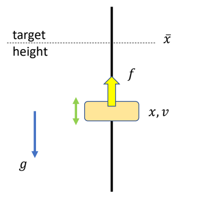
计算一条目标轨迹 \(\tilde{x}(t)\),使得仿真轨迹 \(x(t)\) 是正弦曲线。
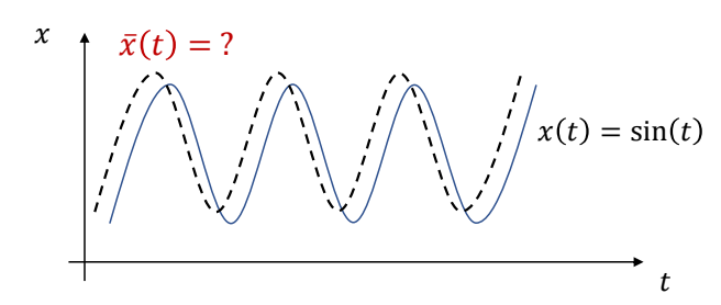
✅ 目标函数是关于优化对象 \(x _n\) 的二次函数。
$$ \min _{(x _n,v _n,\tilde{x} _n)} \sum _{n=0}^{N} (\sin (t _n)-x _n)^2+\sum _{n=0}^{N}\tilde{x} ^2 _n $$
✅ 运动学方程中的 \(x _{n+1}\)、\(v _{n+1}\) 与上一帧状态 \(x _n\)、\(v _n\) 是线性关系。
$$ \begin{aligned} s.t. \quad \quad v _ {n+1} & = v _ n + h(k _p ( \tilde{x} _ n - x _ n) - k _ dv _ n ) \\ x _ {n+1} & = x _ n + hv _ {n+1} \end{aligned} $$
✅ 这是一个典型的 LQR 问题。
动态规划(Dynamic Programming)
LQR 问题使用动态规划方法求解。这部分解释三个核心概念:
1. 什么是动态规划问题?为什么要用动态规划?
动态规划(Dynamic Programming, DP) 是一种求解多阶段决策问题的方法,适用于可以将问题分解为多个 sequential steps 的场景。
为什么 LQR 要用动态规划?
| 原因 | 说明 |
|---|---|
| 问题结构匹配 | LQR 是多阶段决策问题:每个时间步都要选择控制输入 \(a_t\) |
| 全局最优分解 | 动态规划将"找最优轨迹"这个全局问题分解为"每步选最优控制"的局部问题 |
| 高效求解 | 通过逆向递推,可以一次性求出所有时间步的最优策略,无需迭代 |
直观类比:
从 A 点开车到 B 点,如何选择路线?

方法 1:枚举所有可能路线,比较总长度 → 计算量爆炸
方法 2:动态规划 —— 从终点往回推,每个路口选择"到终点最短"的方向 → 高效
在 LQR 中:
- 目标:找到控制序列 \(a_{0:T}\),使总代价最小
- 方法:从最后一步 \(T\) 往前推,每一步求解局部最优
- 结果:得到最优反馈策略 \(a_t^* = -K_t s_t\)
2. 什么是最优子结构?为什么 LQR 具有最优子结构?
最优子结构的定义
Bellman 最优性原理:最优策略具有这样的性质——无论初始状态和初始决策是什么,剩余的决策对于由第一个决策产生的状态而言,必须构成最优策略。
用数学语言表达:
$$ V(s) = \min_{a} \left[ h(s, a) + V(f(s, a)) \right] $$
其中:
- \(V(s)\):从状态 \(s\) 到终点的最小总代价(Value Function)
- \(h(s, a)\):当前步的即时代价
- \(f(s, a)\):状态转移函数
- \(V(f(s, a))\):从下一状态到终点的最小代价
为什么 LQR 具有最优子结构?
LQR 问题满足最优子结构的两个关键条件:
| 条件 | LQR 中的体现 |
|---|---|
| 无后效性 | 下一状态 \(s_{t+1}\) 只取决于当前状态 \(s_t\) 和控制 \(a_t\),与历史无关 |
| 代价可分解 | 总代价是各步代价之和:\(J = \sum (s_t^T Q_t s_t + a_t^T R_t a_t)\) |
直观理解:
时刻:    0 → 1 → 2 → ... → t → t+1 → ... → T
          │         │              │
          └─────────┴──────────────┘
               未来决策只取决于当前状态 s_t
               与之前如何到达 s_t 无关
这意味着:
- 在时刻 \(t\),只需要考虑"从 \(s_t\) 到终点"的最优策略
- 不需要关心"是如何到达 \(s_t\) 的"
- 因此可以从终点 \(T\) 开始,一步步往前推导最优策略
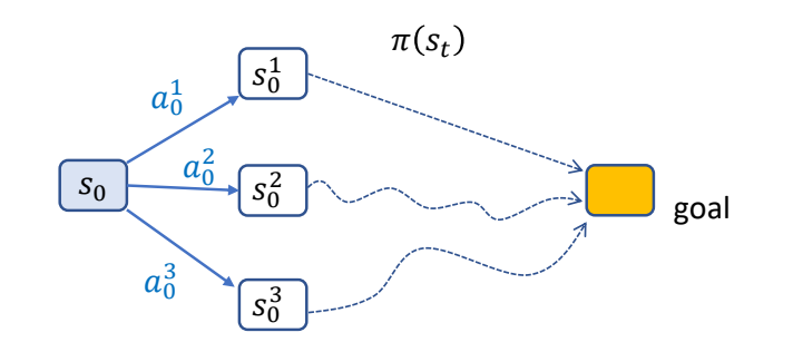
3. 什么是 Value Function?
Value Function 的定义
Value Function(值函数) \(V(s)\) 表示:
从状态 \(s\) 出发,使用最优策略到达终点所需的最小总代价。
$$ V(s) = \min_{a_{0:T}} J(s, a_{0:T}) $$
在 LQR 中,Value Function 具有二次形式:
$$ V_t(s) = s^T P_t s $$
其中 \(P_t\) 是对称矩阵,表示"从时刻 \(t\) 的状态 \(s\) 到终点的代价权重"。
Value Function 的物理意义
| 概念 | 说明 |
|---|---|
| 状态价值 | \(V(s)\) 越小,表示从 \(s\) 出发越"有利"(离目标越近) |
| 未来代价的封装 | \(V(s_t)\) 包含了"从 \(s_t\) 到终点"的所有未来代价 |
| 递推的关键 | 通过 \(V_{t+1}\) 可以推导 \(V_t\),实现逆向动态规划 |
Value Function 的递推关系
根据 Bellman 方程:
$$ V_t(s_t) = \min_{a_t} \left[ \underbrace{s_t^T Q_t s_t + a_t^T R_t a_t}{\text{即时代价}} + \underbrace{V{t+1}(s_{t+1})}_{\text{未来代价}} \right] $$
代入 \(s_{t+1} = A_t s_t + B_t a_t\) 和 \(V_{t+1}(s) = s^T P_{t+1} s\):
$$ V_t(s_t) = \min_{a_t} \left[ s_t^T Q_t s_t + a_t^T R_t a_t + (A_t s_t + B_t a_t)^T P_{t+1} (A_t s_t + B_t a_t) \right] $$
通过求导找到最优 \(a_t^*\),代回得到 \(V_t(s) = s^T P_t s\) 的递推公式(Riccati 方程)。
动态规划求解流程总结
逆向动态规划(Backward Pass)

初始化:P_T = Q_T  (终点的 Value Function)

对 t = T-1, T-2, ..., 0:
    1. 写出 V_t(s) = min [即时代价 + V_{t+1}(s_{t+1})]
    2. 对 a_t 求导,得到最优控制 a_t^* = -K_t s_t
    3. 代回 V_t,得到 P_t 的递推公式(Riccati 方程)
    4. 存储 K_t 和 P_t

结果:
    - 所有时间步的反馈增益 {K_0, K_1, ..., K_{T-1}}
    - 所有时间步的 Value Function 矩阵 {P_0, P_1, ..., P_T}
正向执行(Forward Pass):
$$ \text{对每个 } t: \quad a_t = -K_t s_t $$
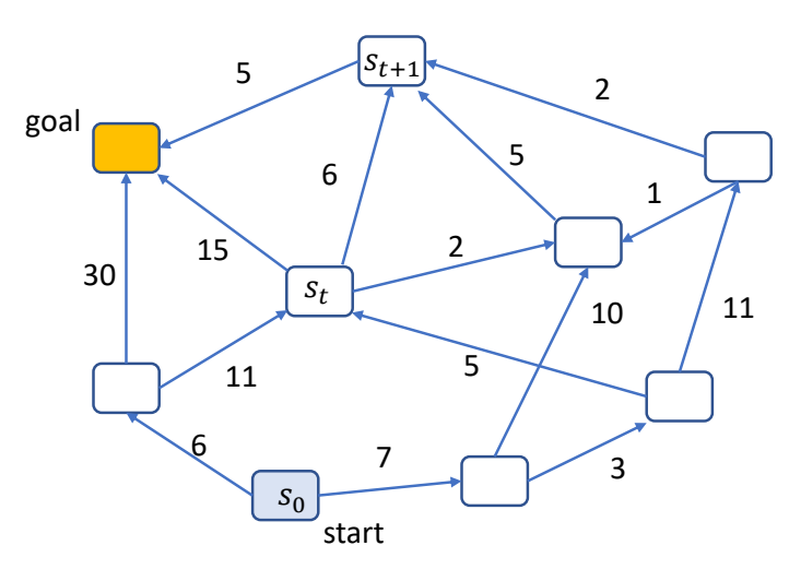
最后一步的推导
考虑最后一步(从 \(T-1\) 到 \(T\)):
$$ V _{T-1}(s _{T-1}) = \min _{a _{T-1}} \left[ s _{T-1}^T Q _{T-1} s _{T-1} + a _{T-1}^T R _{T-1} a _{T-1} + V _T(s _T) \right] $$
代入 \(s _T = A _{T-1} s _{T-1} + B _{T-1} a _{T-1}\) 和 \(V _T(s _T) = s _T^T P _T s _T\):
$$ V _{T-1}(s _{T-1}) = \min _{a _{T-1}} \left[ s _{T-1}^T Q _{T-1} s _{T-1} + a _{T-1}^T R _{T-1} a _{T-1} + (A _{T-1} s _{T-1} + B _{T-1} a _{T-1})^T P _T (A _{T-1} s _{T-1} + B _{T-1} a _{T-1}) \right] $$
求解最优控制
对 \(a _{T-1}\) 求导并令导数为零:
$$ \frac{\partial V _{T-1}}{\partial a _{T-1}} = 2 R _{T-1} a _{T-1} + 2 B _{T-1}^T P _T (A _{T-1} s _{T-1} + B _{T-1} a _{T-1}) = 0 $$
整理得:
$$ (R _{T-1} + B _{T-1}^T P _T B _{T-1}) a _{T-1} = -B _{T-1}^T P _T A _{T-1} s _{T-1} $$
解得最优控制:
$$ a _{T-1}^* = -(R _{T-1} + B _{T-1}^T P _T B _{T-1})^{-1} B _{T-1}^T P _T A _{T-1} s _{T-1} $$
最优控制律的一般形式
$$ a _t^* = -K _t s _t $$
其中反馈增益矩阵 \(K _t\) 为:
$$ K _t = (R _t + B _t^T P _{t+1} B _t)^{-1} B _t^T P _{t+1} A _t $$
✅ 结论:最优策略是当前状态的线性函数,\(K\) 是线性反馈系数。
求解 Value Function
将最优控制 \(a _t^* = -K _t s _t\) 代回 Value Function:
$$ V _{t}(s _t) = s _t^T (Q _t + K _t^T R _t K _t + (A _t - B _t K _t)^T P _{t+1} (A _t - B _t K _t)) s _t $$
因此:
$$ P _t = Q _t + K _t^T R _t K _t + (A _t - B _t K _t)^T P _{t+1} (A _t - B _t K _t) $$
或者展开为更常见的形式(离散代数 Riccati 方程):
$$ P _t = Q _t + A _t^T P _{t+1} A _t - A _t^T P _{t+1} B _t (R _t + B _t^T P _{t+1} B _t)^{-1} B _t^T P _{t+1} A _t $$
✅ \(V(s _{T-1})\) 和 \(V(s _T)\) 的形式基本一致,只是 \(P\) 的表示不同。
逆向递推算法
从终点往起点递推计算 \(P _t\) 和 \(K _t\):
| 步骤 | 计算 |
|---|---|
| 初始化 | \(P _T = Q _T\)(终端代价) |
| 对 \(t = T-1, T-2, \dots, 0\) | |
| 1. 计算反馈增益 | \(K _t = (R _t + B _t^T P _{t+1} B _t)^{-1} B _t^T P _{t+1} A _t\) |
| 2. 更新 P 矩阵 | \(P _t = Q _t + K _t^T R _t K _t + (A _t - B _t K _t)^T P _{t+1} (A _t - B _t K _t)\) |
| 3. 存储 | \(K _t, P _t\) |
Solution 总结
- LQR is a special class of optimal control problems with
- Linear dynamic function
- Quadratic objective function
- Solution of LQR is a linear feedback policy
$$ a _t^* = -K _t s _t $$
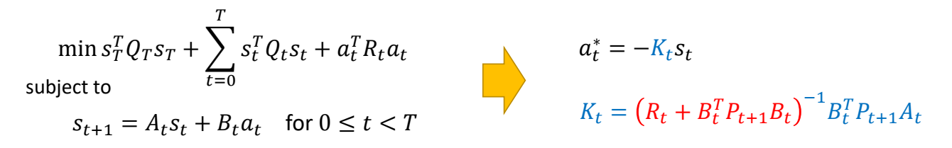
离线计算:从 \(T\) 到 \(0\) 逆向递推,计算所有 \(K _t\)
在线执行:对每个时间步,应用 \(a _t = -K _t s _t\)
更复杂的情况
如何处理非线性问题?
- How to deal with
- Nonlinear dynamic function?
- Non-quadratic objective function?
✅ 人体运动涉及到角度旋转,因此是非线性的。
解决方案:
| 方法 | 核心思想 |
|---|---|
| iLQR | 迭代线性化 + LQR 求解 |
| DDP | 二阶泰勒展开 + 动态规划 |
| CMA-ES | 无导数优化(不需要线性化) |
这些方法将在后续章节介绍。
本文出自 CaterpillarStudyGroup,转载请注明出处。
https://caterpillarstudygroup.github.io/GAMES105_mdbook/
Iterative LQR (iLQR)
✅ 本章定位:理解 iLQR 如何求解非线性轨迹优化问题,掌握其核心思想、算法流程和应用场景。
一、从 LQR 到 iLQR
LQR 的局限性
LQR 问题有闭式解,但仅适用于:
| 假设 | 数学形式 | 限制 |
|---|---|---|
| 线性动力学 | \(x_{t+1} = A_t x_t + B_t u_t\) | 只能处理线性系统 |
| 二次目标函数 | \(J = x_T^T Q_T x_T + \sum (x_t^T Q_t x_t + u_t^T R_t u_t)\) | 代价必须是二次的 |
问题:人形角色动画是非线性系统:
- 关节旋转涉及三角函数
- 动力学方程包含科里奥利力、离心力等非线性项
- 接触约束是非线性的
iLQR 的核心思想
关键洞察:虽然 LQR 只能处理线性系统,但可以在当前轨迹附近局部线性化,然后用 LQR 求解。
非线性轨迹优化问题
    ↓
在当前轨迹 (x̄, ū) 附近线性化
    ↓
δx_{t+1} = A·δx_t + B·δu_t  (线性化动力学)
    ↓
J ≈ δx^T Q δx + δu^T R δu  (二次近似)
    ↓
LQR 问题(有闭式解)
    ↓
求解得到最优控制 δu* = -K·δx
    ↓
更新轨迹:x ← x̄ + δx, u ← ū + δu
    ↓
重复线性化→求解→更新,直到收敛
这就是 iLQR(Iterative LQR)的核心思想!
二、每轮迭代中做了什么
iLQR 的每一轮迭代,本质上就是在当前轨迹处构造一个 LQR 子问题并求解。构造过程涉及三个操作(详细推导见 LQR):
| 操作 | 对 LQR 的意义 | 在 iLQR 中的含义 |
|---|---|---|
| 线性化动力学 | 直接给出 A、B | 在标称轨迹 \((\bar{x}, \bar{u})\) 处计算雅可比 \(A_t = \partial f/\partial x\)、\(B_t = \partial f/\partial u\) |
| 二次化代价 | 直接给出 Q、R | 在标称轨迹处计算 Hessian \(Q_t = \partial^2 J/\partial x^2\)、\(R_t = \partial^2 J/\partial u^2\) |
| 求解 Riccati 方程 | 得到最优反馈 \(u^* = -Kx\) | 得到最优修正量 \(\delta u^* = -K\delta x\) |
关键区别:LQR 里 A、B、Q、R 是问题本身给定的,而 iLQR 里它们每轮都在变——因为线性化点 \((\bar{x}, \bar{u})\) 随着迭代在移动。
修正量 vs 全量
LQR 直接输出最优控制 \(u^* = -Kx\)。iLQR 输出的是修正量:
$$u_{new} = \bar{u} + \alpha \cdot \delta u^* = \bar{u} + \alpha \cdot (-K\delta x)$$
其中 \(\alpha\) 是线搜索步长。直觉上:每次只敢走一小步,避免跳出局部近似的有效范围。
三、iLQR 算法
完整算法流程
算法:iLQR 轨迹优化

输入:
    - 非线性动力学 f(x, u)
    - 目标函数 J(x, u)
    - 初始状态 x₀
    - 初始控制猜测 ū₀:T

输出:
    - 最优状态轨迹 x*₀:T
    - 最优控制轨迹 u*₀:T

步骤:
1. 初始化:设定初始轨迹 (x̄, ū)
2. Repeat until convergence:

   (a) 前向传递(Forward Pass)
       - 用当前控制 ū 仿真得到状态轨迹 x̄
       - 计算当前总代价 J

   (b) 线性化/二次化
       - 计算雅可比矩阵:Aₜ = ∂f/∂x, Bₜ = ∂f/∂u
       - 计算 Hessian 矩阵:Qₜ = ∂²J/∂x², Rₜ = ∂²J/∂u²

   (c) 逆向传递(Backward Pass)
       - 初始化:P_T = Q_T
       - 对 t = T-1, ..., 0:
         · 计算 Kₜ = (Rₜ + BₜᵀPₜ₊₁Bₜ)⁻¹ BₜᵀPₜ₊₁Aₜ
         · 计算 Pₜ = Qₜ + KₜᵀRₜKₜ + (Aₜ - BₜKₜ)ᵀPₜ₊₁(Aₜ - BₜKₜ)
         · (可选)计算 feedforward 项 kₜ

   (d) 更新控制
       - 计算新控制:u_new = ū + α·δu* (α 为线搜索步长)
       - δu* = -K·δx + k (LQR 解)

   (e) 收敛检查
       - 如果 |J_new - J| < ε,则收敛
前向传递 vs 逆向传递
| 步骤 | 目的 | 输入 | 输出 |
|---|---|---|---|
| 前向传递 | 仿真轨迹、计算代价 | 控制轨迹 ū | 状态轨迹 x̄、代价 J |
| 线性化 | 局部近似为 LQR 问题 | 轨迹 (x̄, ū) | 矩阵 A, B, Q, R |
| 逆向传递 | 求解 LQR、计算最优策略 | 矩阵 A, B, Q, R | 反馈增益 K、Value 矩阵 P |
| 更新 | 改进轨迹 | K, 当前轨迹 | 新控制轨迹 |
算法可视化
迭代 1: 初始轨迹(可能不满足动力学)
    ↓
┌─────────────────────────────┐
│  前向传递:仿真得到 x̄        │
│  线性化:计算 A, B           │
│  逆向传递:计算 K            │
│  更新:u_new = u + δu*      │
└─────────────────────────────┘
    ↓
迭代 2: 改进的轨迹
    ↓
┌─────────────────────────────┐
│  重复...                    │
└─────────────────────────────┘
    ↓
迭代 N: 收敛到最优轨迹
四、iLQR 与 DDP 的对比
一阶 vs 二阶方法
| 方法 | 动力学近似 | 目标函数近似 | 梯度需求 | 收敛速度 |
|---|---|---|---|---|
| iLQR | 一阶泰勒展开 | 二阶泰勒展开 | 一阶导数 | 线性收敛 |
| DDP | 二阶泰勒展开 | 二阶泰勒展开 | 二阶导数 | 二阶收敛 |
数学差异
iLQR(一阶动力学): $$ f(x,u) \approx f(\bar{x},\bar{u}) + \nabla f(\bar{x},\bar{u}) \begin{bmatrix} x-\bar{x} \ u-\bar{u} \end{bmatrix} $$
DDP(二阶动力学): $$ f(x,u) \approx f(\bar{x},\bar{u}) + \nabla f(\bar{x},\bar{u}) \begin{bmatrix} x-\bar{x} \ u-\bar{u} \end{bmatrix} + \frac{1}{2} \begin{bmatrix} x-\bar{x} \ u-\bar{u} \end{bmatrix}^T \nabla^2 f(\bar{x},\bar{u}) \begin{bmatrix} x-\bar{x} \ u-\bar{u} \end{bmatrix} $$
方法选择
| 场景 | 推荐方法 | 原因 |
|---|---|---|
| 平滑非线性问题 | iLQR | 一阶导数易计算,收敛快 |
| 高精度需求 | DDP | 二阶收敛,迭代次数少 |
| 动力学复杂 | iLQR | 避免计算二阶导数 |
| 接触频繁 | 其他方法 | iLQR/DDP 都需可微模型 |
五、iLQR 在轨迹优化中的定位
按分类维度
| 维度 | iLQR 的定位 |
|---|---|
| 优化时机 | 离线/在线均可 |
| 求解方法 | 数值法(迭代) |
| 梯度需求 | 基于梯度(一阶) |
| 适用系统 | 非线性(通过线性化) |
| 适用场景 | 平滑非线性问题 |
与其他方法对比
| 方法 | 时机 | 梯度 | 闭式解 | 适用场景 |
|---|---|---|---|---|
| LQR | 离线/在线 | N/A | ✅ | 线性系统 |
| iLQR | 离线/在线 | 一阶 | ⚠️ 每轮闭式 | 平滑非线性 |
| DDP | 离线/在线 | 二阶 | ⚠️ 每轮闭式 | 高精度需求 |
| CMA-ES | 离线 | 零阶 | ❌ | 非凸/不可微 |
| SAMCON | 在线 | 零阶 | ❌ | 角色实时控制 |
方法选择建议
更多方法对比请参见:方法对比与分类。
问题类型 → 推荐方法
─────────────────────────
线性系统 → LQR
平滑非线性 → iLQR/DDP
接触频繁/不可微 → CMA-ES
实时控制 → MPC/SAMCON
需要泛化 → DeepMimic/AMP
离线制作动作 → iLQR/DDP/CMA-ES
六、工程实践
应用实例
| 应用 | 说明 |
|---|---|
| 轨迹跟踪 | 用动捕数据作为参考,优化出物理可行的轨迹 |
| 局部修正 | 在现有轨迹附近优化,应对扰动 |
| 动作生成 | 结合前馈 + 反馈控制,生成平滑动作 |
实际考虑
1. 初始猜测的重要性
- iLQR 是局部优化方法,可能陷入局部最优
- 好的初始猜测(如动捕数据)能显著提高结果质量
2. 线搜索(Line Search)
- 更新轨迹时需要控制步长 α
- 常用:Armijo 条件、回溯线搜索
3. 正则化
- 在 Hessian 矩阵上加正则项防止奇异
- \(R \leftarrow R + \lambda I\)
4. 终止条件
- 代价变化小于阈值:\(|J_{new} - J| < \epsilon\)
- 达到最大迭代次数
七、与 DeepMimic/AMP 的关系
| 维度 | iLQR | DeepMimic/AMP |
|---|---|---|
| 输出 | 单一轨迹 \(\mathbf{x} _{0:T}\) | 策略 \(\pi(\mathbf{a} |
| 计算时机 | 离线优化(每任务一次) | 训练一次,在线推理 |
| 泛化能力 | 无(仅适用于该轨迹) | 有(可处理新情况) |
| 计算成本 | 中(秒级) | 低(毫秒级推理) |
| 适用场景 | 特定动作生成 | 通用角色控制 |
关系:
- iLQR 轨迹优化结果可作为 RL 的参考轨迹
- RL 可学习模仿 iLQR 生成的行为
八、关键要点总结
核心思想
- 迭代线性化:在当前位置附近将非线性问题近似为 LQR 问题
- 前后向传递:前向仿真轨迹,逆向求解最优策略
- 闭式解:每轮迭代都有 LQR 闭式解,但需要多次迭代收敛
算法流程
初始化轨迹 → 前向传递 → 线性化 → 逆向传递 → 更新轨迹 → 检查收敛
优缺点
| 优点 | 缺点 |
|---|---|
| 收敛快(相比无梯度方法) | 需要可微模型 |
| 适用于高维问题 | 可能陷入局部最优 |
| 每轮迭代有闭式解 | 计算雅可比矩阵成本高 |
适用场景
- ✅ 平滑的非线性轨迹优化问题
- ✅ 有参考轨迹的跟踪问题
- ✅ 需要精确控制的场景
- ❌ 接触频繁、不可微的问题(用 CMA-ES)
- ❌ 实时控制(用 MPC/SAMCON)
九、深入学习
前置知识
相关方法
参考资料
- Muico et al 2011 - Composite Control of Physically Simulated Characters
- Al Borno et al. 2013 - Trajectory Optimization for Full-Body Movements with Complex Contacts
本文出自 CaterpillarStudyGroup,转载请注明出处。 https://caterpillarstudygroup.github.io/GAMES105_mdbook/
Differential Dynamic Programming (DDP)
✅ 本章定位:理解 DDP 如何在 iLQR 的基础上引入二阶动力学近似,实现更快的收敛速度;掌握 DDP 与 iLQR 的精确差异和各自的适用场景。
一、DDP 的核心思想
从 iLQR 到 DDP
iLQR 在每轮迭代中将非线性动力学做一阶泰勒展开,然后解一个 LQR 子问题。DDP 的做法几乎完全一样,唯一的区别在于:
对动力学也做二阶泰勒展开。
这意味着 DDP 在构造局部近似时,不仅考虑了动力学的梯度方向(一阶),还考虑了动力学的曲率信息(二阶),因此每步近似更精确,收敛更快。
iLQR:  δx_{t+1} ≈ A·δx + B·δu                          (一阶动力学)
DDP:   δx_{t+1} ≈ A·δx + B·δu + ½·[δx,δu]ᵀ·C·[δx,δu]   (二阶动力学)
其中 C 是动力学的 Hessian 张量。
二、与 iLQR 的精确差异
构造 LQR 子问题的三个操作
| 操作 | iLQR | DDP |
|---|---|---|
| 线性化动力学 | 一阶泰勒:A = ∂f/∂x,B = ∂f/∂u | 二阶泰勒:额外计算 C = ∂²f/∂(x,u)² |
| 二次化代价 | 二阶泰勒:Q、R | 二阶泰勒:Q、R(与 iLQR 相同) |
| 求解 Riccati 方程 | 标准形式 | 需要额外修正项来吸收二阶动力学项 |
二阶动力学带来的代价
DDP 在逆向传递中需要处理二阶动力学项。将二阶展开代入 Riccati 方程后,会多出一项涉及动力学 Hessian 的修正:
$$V_x'(x) = V_x(f(x,u)) + V_{xx}(f(x,u)) \cdot f_x(x,u)$$
$$V_{xx}'(x) = f_x(x,u)^T V_{xx} f(x,u) + V_{xx}(f(x,u)) \cdot f_{xx}(x,u) + l_{xx}(x,u)$$
其中 f_{xx} 就是动力学的二阶导数——iLQR 完全忽略了这一项。
梯度需求对比
| 导数 | iLQR 是否需要 | DDP 是否需要 | 计算成本 |
|---|---|---|---|
| ∂f/∂x(雅可比) | ✅ | ✅ | 中 |
| ∂f/∂u(雅可比) | ✅ | ✅ | 中 |
| ∂²f/∂x²(Hessian) | ❌ | ✅ | 高 |
| ∂²f/∂u²(Hessian) | ❌ | ✅ | 高 |
| ∂²f/∂x∂u(交叉 Hessian) | ❌ | ✅ | 高 |
三、收敛性差异
理论保证
| 性质 | iLQR | DDP |
|---|---|---|
| 收敛阶数 | 线性收敛(一阶) | 二次收敛(二阶) |
| 每轮计算量 | 较低(只算雅可比) | 较高(需算 Hessian) |
| 总迭代次数 | 较多 | 较少(通常 2-3 倍差距) |
直觉:iLQR 每步走的方向大致正确但步长受限于线性近似的精度;DDP 因为有曲率信息,不仅能走更精确的方向,还能自适应调整步长。
实际选择
问题特征 → 推荐方法
─────────────────────
动力学平滑、二阶导容易算 → DDP(总时间更短)
动力学复杂、二阶导计算昂贵 → iLQR(每轮更快)
对精度要求极高 → DDP
需要鲁棒性(不依赖精确二阶导) → iLQR
四、算法流程
DDP 的算法流程与 iLQR 几乎完全一致,区别仅在于逆向传递:
算法:DDP 轨迹优化

输入/输出:同 iLQR

步骤:
1. 初始化:设定初始轨迹 (x̄, ū)
2. Repeat until convergence:

   (a) 前向传递
       - 用当前控制 ū 仿真得到状态轨迹 x̄
       - 计算当前总代价 J

   (b) 计算 Jacobian 和 Hessian
       - 一阶:Aₜ = ∂f/∂x,  Bₜ = ∂f/∂u        ← 与 iLQR 相同
       - 二阶:Cₜ = ∂²f/∂(x,u)²                 ← DDP 额外需要

   (c) 逆向传递(含二阶修正)
       - 初始化:Vₓ = lₓ,  Vₓₓ = lₓₓ
       - 对 t = T-1, ..., 0:
         · 计算 Qₓ, Qᵤ, Qₓₓ, Qᵤᵤ, Qₓᵤ(含动力学二阶修正项)
         · 计算 kₜ(feedforward), Kₜ(feedback gain)
         · 更新 Value 函数导数 Vₓ, Vₓₓ(含 fₓₓ 修正项)  ← DDP 的关键区别

   (d) 线搜索 + 更新控制
       - u_new = ū + α·(k + K·δx)

   (e) 收敛检查
与 iLQR 逆向传递的唯一区别:Vₓₓ 的更新公式中多了 Vₓₓ · fₓₓ 这一项(动力学 Hessian 对 Value 函数 Hessian 的贡献)。
五、iLQR 与 DDP 的关系总结
LQR(线性系统,一次求解)
 │
 ├─ 加一层迭代 + 一阶线性化 → iLQR(非线性系统,线性收敛)
 │
 └─ 加一层迭代 + 二阶线性化 → DDP(非线性系统,二次收敛)
两者的关系可以概括为:
| LQR | iLQR | DDP | |
|---|---|---|---|
| 系统类型 | 线性 | 非线性 | 非线性 |
| 动力学近似阶数 | 精确(本身就是线性) | 一阶 | 二阶 |
| 代价近似阶数 | 精确(本身就是二次) | 二阶 | 二阶 |
| 是否需要迭代 | ❌ | ✅ | ✅ |
| 每轮闭式解 | ✅ | ✅ | ✅(修正后) |
| 收敛速度 | N/A | 线性 | 二次 |
| 核心瓶颈 | 仅限线性系统 | 一阶近似的精度 | 二阶导的计算成本 |
六、工程实践
DDP 的常见问题
1. Hessian 计算成本
- 对于解析可微的动力学(如刚体),可以用自动微分或符号推导
- 对于黑箱仿真器,需要用有限差分近似,成本随状态维度平方增长
2. 数值稳定性
- 二阶项可能使 Hessian 不定(非正定),导致下降方向不可靠
- 常用 Levenberg-Marquardt 正则化:在 Hessian 对角线加 λI
3. iLQR 实际上更常用
- 在角色动画领域,iLQR 的使用频率远高于 DDP
- 原因:大多数物理仿真器的二阶导数难以获取,而 iLQR 的一阶近似在大多数场景下已经足够
七、深入学习
前置知识
相关方法
参考资料
- Mayne, D. Q. (1966). A Second-Order Solution of the Optimal Control Problem. (DDP 的原始论文)
- Tassa, Y., Mansard, N., & Todorov, E. (2012). Control-Limited Differential Dynamic Programming. (带控制约束的 DDP)
本文出自 CaterpillarStudyGroup,转载请注明出处。 https://caterpillarstudygroup.github.io/GAMES105_mdbook/
Model Predictive Control (MPC)
✅ 本章定位:理解 MPC 如何通过滚动时域优化实现闭环最优控制,掌握其核心思想、算法流程和在角色动画中的应用。
⭐ 核心概念:MPC 是一个控制框架
MPC 本身不是一个具体的优化算法,而是一个控制框架。
它定义了**"每帧优化、只执行第一步、然后重新优化"的闭环控制思想,但不指定具体用什么方法求解**优化问题。
MPC 框架 + 不同求解器
MPC 框架(滚动时域优化)
    │
    ├─ 结合 iLQR 求解器  →  iLQR-MPC(适用于平滑问题)
    │
    ├─ 结合 DDP 求解器   →  DDP-MPC(适用于高精度需求)
    │
    ├─ 结合 CMA-ES      →  Sampling-MPC(适用于不可微问题)
    │
    ├─ 结合 SAMCON      →  粒子滤波 MPC(适用于角色控制)
    │
    └─ 结合凸优化       →  Convex-MPC(适用于凸问题)
| 组件 | 作用 | 类比 |
|---|---|---|
| MPC 框架 | 定义"何时优化、如何执行" | 汽车的"自动驾驶系统" |
| 求解器 | 实际计算最优控制 | 汽车的"发动机"(可以是汽油、柴油、电动) |
重要理解:
- MPC 的核心是滚动时域思想,不是某个特定算法
- 同一个 MPC 框架,换不同求解器,适用于不同问题
- 选择求解器时要考虑:可微性、计算成本、精度需求
一、从开环到闭环:为什么需要 MPC
开环控制的局限性
前面介绍的轨迹优化方法(如 iLQR、DDP、CMA-ES)主要是开环控制:
离线优化一次 → 得到最优轨迹 (x*, u*) → 执行
| 优点 | 缺点 |
|---|---|
| 可预先计算、推理快 | 无法应对扰动 |
| 适用于动作生成 | 误差会累积 |
| 计算成本一次性投入 | 实际轨迹可能偏离规划 |
问题:角色动画中经常遇到扰动:
- 外力推挤
- 地面不平
- 模型参数误差
- 数值仿真误差累积
闭环控制的思想
反馈控制:每帧根据当前状态重新计算控制
测量当前状态 s → 查表 u = -K·s → 执行 → 下一帧
PD 控制就是典型的闭环控制,但它是局部的:
- 只考虑当前状态与目标状态的偏差
- 不考虑未来、不预测后果
- 无法处理复杂约束
MPC 的核心洞察
MPC = 开环优化 + 闭环执行
每帧都做一次开环轨迹优化,但只执行第一步,然后重新优化
t=0: 测量 s₀ → 优化得到 (u₀*, u₁*, ..., uₙ*) → 执行 u₀*
t=1: 测量 s₁ → 优化得到 (u₀*, u₁*, ..., uₙ*) → 执行 u₀*
t=2: 测量 s₂ → 优化得到 (u₀*, u₁*, ..., uₙ*) → 执行 u₀*
...
关键:
- 每帧都基于最新测量状态重新规划
- 只执行规划序列的第一步
- 下一帧重复优化,形成反馈
二、MPC 的数学描述
标准 MPC 问题
在每一时刻 t,求解如下优化问题:
$$ \begin{aligned} \min_{\mathbf{u}_{0:N-1}} \quad & \phi(\mathbf{x}N) + \sum{k=0}^{N-1} \ell(\mathbf{x}_k, \mathbf{u}k) \ \text{s.t.} \quad & \mathbf{x}{k+1} = f(\mathbf{x}_k, \mathbf{u}_k) \quad \text{(动力学)} \ & \mathbf{x}0 = \mathbf{x}{\text{current}} \quad \text{(当前状态)} \ & \mathbf{x}_k \in \mathcal{X}, \mathbf{u}_k \in \mathcal{U} \quad \text{(约束)} \end{aligned} $$
其中:
- \(N\):预测时域(Prediction Horizon),通常 10-50 步
- \(\phi(\mathbf{x}_N)\):终端代价
- \(\ell(\mathbf{x}_k, \mathbf{u}_k)\):阶段代价
- \(\mathcal{X}, \mathcal{U}\):状态和控制约束集
MPC 算法流程
算法:MPC 闭环控制

输入:
    - 当前状态 x_current
    - 参考轨迹 x_ref
    - 预测时域 N

输出:
    - 控制输入 u*

每帧执行:
1. 测量当前状态 x_current

2. 求解优化问题:
   min J = φ(x_N) + Σₖ₌₀ᴺ⁻¹ ℓ(x_k, u_k)
   s.t. x_{k+1} = f(x_k, u_k)
        x_0 = x_current
        x_k ∈ X, u_k ∈ U

3. 得到最优控制序列 (u₀*, u₁*, ..., uₙ*₋₁)

4. 执行第一步控制 u* = u₀*

5. 等待下一帧,回到步骤 1
与开环优化的对比
| 维度 | 开环优化 (iLQR, DDP) | MPC |
|---|---|---|
| 优化频率 | 一次(离线) | 每帧(在线) |
| 输入状态 | 固定初始状态 x₀ | 实时测量 x_current |
| 执行方式 | 执行完整轨迹 | 只执行第一步 |
| 应对扰动 | ❌ 无法应对 | ✅ 自动校正 |
| 计算成本 | 一次性高 | 持续高 |
| 适用场景 | 动作生成/离线规划 | 实时控制/跟踪 |
三、MPC 的关键设计要素
1. 预测时域 (Prediction Horizon)
预测时域 \(N\) 的选择是 MPC 设计的核心:
| 时域长度 | 优点 | 缺点 | 适用场景 |
|---|---|---|---|
| 短 (N=5-10) | 计算快 | 短视、可能不稳定 | 快速反应任务 |
| 中 (N=10-30) | 平衡 | 中等计算量 | locomotion、跟踪 |
| 长 (N=30-100) | 远视、稳定 | 计算慢 | 复杂规划任务 |
经验法则:
- 时域应覆盖任务的关键动态
- 例如:走路步态周期约 1 秒,若 dt=0.01s,则 N≈100
2. 代价函数设计
MPC 的代价函数通常包含:
$$ J = J_{\text{track}} + J_{\text{control}} + J_{\text{smooth}} + J_{\text{terminal}} $$
| 项 | 数学形式 | 作用 |
|---|---|---|
| 跟踪误差 | \(\sum (\mathbf{x}_k - \mathbf{x}_k^{\text{ref}})^T Q (\mathbf{x}_k - \mathbf{x}_k^{\text{ref}})\) | 跟踪参考轨迹 |
| 控制 effort | \(\sum \mathbf{u}_k^T R \mathbf{u}_k\) | 避免过大控制 |
| 平滑项 | \(\sum (\mathbf{u}k - \mathbf{u}{k-1})^T S (\mathbf{u}k - \mathbf{u}{k-1})\) | 控制变化平滑 |
| 终端代价 | \(\mathbf{x}_N^T P \mathbf{x}_N\) | 保证稳定性 |
3. 约束处理
MPC 的核心优势之一是能显式处理约束:
| 约束类型 | 数学形式 | 示例 |
|---|---|---|
| 状态约束 | \(\mathbf{x} \in \mathcal{X}\) | 关节角度限制、速度限制 |
| 控制约束 | \(\mathbf{u} \in \mathcal{U}\) | 关节力矩上限 |
| 接触约束 | \(g(\mathbf{x}) \geq 0\) | 足部不穿透地面、摩擦锥 |
| 任务约束 | \(h(\mathbf{x}) = 0\) | 手部保持抓握、视线跟踪 |
4. 终端设计
为保证 MPC 稳定性,通常需要设计终端约束或终端代价:
| 方法 | 说明 | 优缺点 |
|---|---|---|
| 终端代价 | \(\phi(\mathbf{x}_N) = \mathbf{x}_N^T P \mathbf{x}_N\) | 软约束,计算简单 |
| 终端约束 | \(\mathbf{x}N = \mathbf{x}{\text{goal}}\) | 硬约束,可能无解 |
| 终端集合 | \(\mathbf{x}_N \in \mathcal{X}_f\) | 灵活但设计复杂 |
| 无终端 | 不设终端 | 简单但可能不稳定 |
四、MPC 的求解方法
核心理解:MPC 是一个框架,它需要调用具体的求解器来解优化问题。
求解器对比
| 求解器类型 | 代表方法 | 特点 | 适用场景 |
|---|---|---|---|
| 基于梯度 | iLQR, DDP, SQP | 收敛快,需要可微模型 | 平滑问题、精确跟踪 |
| 无梯度 | CMA-ES | 不需要梯度,收敛慢 | 非凸问题、接触频繁 |
| 采样方法 | SAMCON, MPPI | 平衡效率和适用性 | 角色控制、复杂约束 |
| 凸优化 | Convex-MPC | 全局最优、高效 | 可公式化为凸问题 |
1. iLQR-MPC(最常用)
在角色动画中最常用的是 iLQR 作为 MPC 的内部求解器:
每帧:
    1. 测量当前状态 x_current
    2. 以 x_current 为初值,运行 iLQR 优化
    3. 得到最优控制序列 (u₀*, u₁*, ..., uₙ*₋₁)
    4. 执行 u₀*
优点:
- 收敛快(适合实时)
- 适用于平滑非线性问题
- 可处理高维系统(如全身角色)
缺点:
- 需要可微模型
- 接触处理困难(需要光滑近似)
2. Sampling-based MPC
对于不可微问题(如接触),可使用采样方法:
SAMCON (Sampling-based Model Predictive Control):
- 在控制空间采样多条轨迹
- 评估每条轨迹的代价
- 选择最优轨迹的第一步执行
- 用 CMA-ES 迭代优化采样分布
MPPI (Model Predictive Path Integral):
- 基于重要性采样的随机 MPC
- 适用于连续控制和随机系统
3. 其他求解器
| 求解器 | 说明 | 适用场景 |
|---|---|---|
| DDP-MPC | 使用 DDP 作为求解器,二阶收敛 | 高精度需求、可计算二阶导数 |
| Convex-MPC | 将问题公式化为凸优化 | 足式机器人、简化模型 |
| NMPC (Nonlinear MPC) | 直接求解非线性优化问题 | 一般非线性系统 |
求解器选择建议
问题特征 → 推荐求解器
─────────────────────────
平滑、可微模型 → iLQR-MPC ⭐
需要二阶精度 → DDP-MPC
接触频繁、不可微 → Sampling-MPC (SAMCON/CMA-ES)
简化模型、凸问题 → Convex-MPC
3. 显式 MPC vs 隐式 MPC
| 类型 | 方法 | 特点 |
|---|---|---|
| 隐式 MPC | 在线求解优化问题 | 灵活、计算量大 |
| 显式 MPC | 离线计算策略表,在线查表 | 快、但存储大、维度低 |
角色动画中主要使用隐式 MPC。
五、MPC 在角色动画中的应用
1. 轨迹跟踪 (Reference Tracking)
问题:给定参考轨迹(动捕数据),让仿真角色跟踪
MPC 方案:
- 状态:关节位置 + 速度
- 控制:关节力矩
- 代价:跟踪误差 + 控制 effort
- 约束:关节限制、力矩限制
优势:
- 自动应对扰动(被推后恢复平衡)
- 可处理模型误差
- 实时性能
2. 平衡控制 (Balance Control)
问题:让角色在不平坦地面上保持平衡
MPC 方案:
- 状态:质心位置 + 速度 + 关节状态
- 控制:关节力矩 + 接触力
- 代价:质心高度 + 基座姿态 + 控制 effort
- 约束:接触力(摩擦锥)、ZMP 约束
3. 步态生成 (Locomotion)
问题:让角色按期望速度行走/跑步
MPC 方案:
- 状态:全身关节状态 + 基座状态
- 控制:关节力矩 + 下一步落脚点
- 代价:速度跟踪 + 能量 + 步态稳定性
- 约束:接触时序、落脚点可行区域
代表性工作:
- Winkler et al. 2020 - 全身 MPC 用于双足行走
- Kim et al. 2019 - MPC 用于复杂地形 locomotion
4. 全身控制 (Whole-Body Control)
问题:同时控制手、脚、基座完成多任务
MPC 方案:
- 状态:全身 50+DoF
- 控制:全身关节力矩
- 代价:多任务加权(手跟踪 + 脚跟踪 + 平衡)
- 约束:全身动力学 + 接触约束
挑战:
- 高维(计算量大)
- 接触切换(混合系统)
- 实时性要求高
六、MPC 与其他方法的对比
MPC vs PID/PD 控制
| 维度 | PD 控制 | MPC |
|---|---|---|
| 优化范围 | 局部(当前误差) | 全局(预测时域内) |
| 约束处理 | 无法显式处理 | 显式处理 |
| 多任务协调 | 难(需要调权重) | 易(统一优化) |
| 计算成本 | 极低 | 高 |
| 适用场景 | 简单跟踪 | 复杂任务 |
MPC vs 轨迹优化
| 维度 | 轨迹优化 (iLQR, DDP) | MPC |
|---|---|---|
| 优化频率 | 一次(离线) | 每帧(在线) |
| 初值敏感性 | 高(可能局部最优) | 低(热启动) |
| 实时性 | 否 | 是 |
| 应对扰动 | 否 | 是 |
| 关系 | MPC 可以用轨迹优化作为求解器 |
MPC vs 强化学习
| 维度 | MPC | 强化学习 |
|---|---|---|
| 训练需求 | 无需训练 | 需要大量训练 |
| 泛化能力 | 有限 | 强 |
| 推理速度 | 慢(ms 级) | 快(μs 级) |
| 可解释性 | 高 | 低 |
| 约束处理 | 显式 | 隐式(需特殊设计) |
| 适用场景 | 已知模型、高精度 | 未知模型、泛化需求 |
方法选择建议
场景 → 推荐方法
─────────────────────────
已知模型 + 实时控制 → MPC
已知模型 + 离线动作 → iLQR/DDP/CMA-ES
未知模型 + 泛化需求 → 强化学习
简单跟踪 → PD 控制
七、MPC 的优缺点
优点
| 优点 | 说明 |
|---|---|
| 闭环最优 | 每帧重新优化,自动应对扰动 |
| 约束处理 | 显式处理状态/控制/接触约束 |
| 多任务协调 | 统一框架下优化多目标 |
| 模型利用 | 充分利用已知模型信息 |
| 灵活性 | 代价函数和约束可在线修改 |
缺点
| 缺点 | 说明 |
|---|---|
| 计算成本高 | 每帧需解优化问题 |
| 模型依赖 | 模型不准会导致性能下降 |
| 调参复杂 | 时域、权重、约束需要调节 |
| 接触处理 | 离散接触需要特殊处理 |
| 稳定性分析 | 理论保证需要终端设计 |
八、工程实践
1. 计算优化
热启动 (Warm Start):
- 用上一帧的解作为当前帧优化的初值
- 显著减少迭代次数
并行化:
- 采样方法可并行评估多条轨迹
- GPU 加速动力学计算
简化模型:
- 使用简化的动力学模型(如线性倒立摆)
- 在简化的控制空间优化
2. 稳定性设计
终端代价:
- 用 LQR 的 Value Function 作为终端代价
- 保证闭环稳定性
足够长的时域:
- 时域应覆盖系统的主要动态
- 经验:至少覆盖一个步态周期
约束松弛:
- 硬约束可能导致无解
- 用软约束(加惩罚)代替
3. 接触处理
光滑近似:
- 用 sigmod 近似接触力的开启/关闭
- 使问题可微
混合 MPC:
- 显式枚举接触模式
- 每种模式下分别优化
分层 MPC:
- 高层规划接触时序
- 低层优化连续轨迹
九、MPC 在 GAMES105 中的定位
与其他方法的关系
轨迹优化方法图谱

按优化时机:
├── 离线优化
│   ├── CMA-ES (无梯度)
│   ├── iLQR (一阶梯度)
│   └── DDP (二阶梯度)
│
└── 在线优化
    ├── MPC (滚动时域)
    │   ├── iLQR-MPC
    │   ├── Sampling-MPC (如 SAMCON)
    │   └── Convex-MPC
    │
    └── 即时反馈
        └── PD 控制
在课程体系中的位置
| 先修内容 | 后续内容 |
|---|---|
| 轨迹优化的数学描述 | SAMCON - 采样-based MPC |
| LQR - 线性最优控制 | SIMBICON - 简化模型预测 |
| iLQR - 非线性轨迹优化 | Character Control |
十、关键要点总结
核心思想
- 滚动时域优化:每帧基于当前状态重新优化未来 N 步
- 只执行第一步:形成闭环反馈
- 显式约束处理:统一框架处理状态/控制/接触约束
MPC 设计要素
| 要素 | 设计考虑 |
|---|---|
| 预测时域 | 平衡计算成本和远视性 |
| 代价函数 | 跟踪 + 控制 + 平滑 + 终端 |
| 约束 | 状态限制 + 控制限制 + 接触 |
| 求解器 | iLQR/SQP/CMA-ES/采样方法 |
优缺点
| 优点 | 缺点 |
|---|---|
| 闭环最优、应对扰动 | 计算成本高 |
| 显式约束处理 | 模型依赖 |
| 多任务协调 | 调参复杂 |
适用场景
- ✅ 实时控制 + 已知模型
- ✅ 需要应对扰动的场景
- ✅ 复杂约束处理
- ❌ 无模型场景(用 RL)
- ❌ 超高频率控制(用 PD)
十一、深入学习
前置知识
- 轨迹优化的数学形式化描述
- LQR - 线性二次调节器
- iLQR - 迭代 LQR
相关方法
参考资料
教程:
论文:
- Rawlings & Mayne 2009 - Model Predictive Control: Theory and Design (教材)
- Winkler et al. 2020 - Convex Model Predictive Control for Bipedal Walking
- Kim et al. 2019 - Reinforcement Learning for Robust Parameterized Locomotion Control
代码:
本文出自 CaterpillarStudyGroup,转载请注明出处。 https://caterpillarstudygroup.github.io/GAMES105_mdbook/
CMA-ES(协方差矩阵自适应进化策略)
✅ 本章定位:理解 无梯度优化方法 在轨迹优化中的应用,掌握 CMA-ES 的核心思想、算法流程和在角色动画中的实际应用。
一、为什么需要无梯度优化?
基于梯度方法的局限
在轨迹优化中,基于梯度的方法(如 iLQR、DDP)需要:
| 要求 | 问题 |
|---|---|
| 可微的动力学模型 | 接触、碰撞等不连续事件不可微 |
| 可微的目标函数 | 某些任务指标不可微 |
| 良好的梯度信息 | 非凸问题容易陷入局部最优 |
现实问题:
- 人形角色动画涉及接触约束(脚与地面接触/离开)
- 目标函数可能高度非凸(多峰、不连续)
- 仿真器通常是黑盒系统,无法提供解析梯度
无梯度方法的优势
| 优势 | 说明 |
|---|---|
| 无需梯度 | 适用于不可微、不连续问题 |
| 黑盒优化 | 只需输入输出,不关心内部机制 |
| 全局搜索 | 更有可能跳出局部最优 |
| 稳定可靠 | 对噪声和不确定性鲁棒 |
代表方法:
- CMA-ES(协方差矩阵自适应进化策略)
- 贝叶斯优化
- 序列蒙特卡洛方法
二、CMA-ES 核心思想
基本概念
CMA-ES (Covariance Matrix Adaptation Evolution Strategy) 是一种进化策略,属于进化计算的分支。
核心思想:
将优化变量建模为高斯分布,通过迭代采样和选择,自适应地更新分布的均值和协方差矩阵,使分布逐渐收敛到最优解。
算法框架
目标:找到变量 x 使目标函数 f(x) 最小

1. 初始化高斯分布:x ~ N(μ, Σ)
   - μ: 均值(当前最优估计)
   - Σ: 协方差矩阵(搜索方向和步长)

2. Repeat until convergence:
   (a) 采样:生成候选解 {x₁, x₂, ..., x_λ} ~ N(μ, Σ)
   (b) 评估:计算每个候选解的目标值 {f(x₁), f(x₂), ..., f(x_λ)}
   (c) 选择:保留前 N 个最优样本(精英样本)
   (d) 更新:根据精英样本更新 μ 和 Σ

3. 输出:最优均值 μ*
可视化理解
迭代 1: 初始分布(大方差,探索阶段)
        o
      o o o
    o  *  o      * = 均值 μ
      o o o        o = 采样点
        o

        ↓ 评估 + 选择 + 更新

迭代 2: 分布向最优方向移动(协方差开始适应)
            o
          o o
        o  * →
          o o
            o

        ↓ 继续迭代

迭代 N: 收敛到最优解(小方差,开发阶段)
          ***
         *****
        *******   * = 密集的最优解区域
三、CMA-ES 算法详解
3.1 初始化
均值向量 \(\mu _0\):
- 可以随机初始化
- 或使用启发式方法(如参考轨迹)
协方差矩阵 \(\Sigma _0\):
- 通常初始化为单位矩阵:\(\Sigma _0 = I\)
- 或根据问题先验知识设置
超参数:
- \(\lambda\):每代采样数量(通常 \(\lambda = 4 + \lfloor 3 \ln n \rfloor\))
- \(\mu\):精英样本数量(通常 \(\mu = \lfloor \lambda/2 \rfloor\))
- \(w _i\):样本权重(通常对数权重)
3.2 采样过程
从多元高斯分布中采样:
$$ x_i ^{(g+1)} \sim \mathcal{N}(\mu ^{(g)}, \Sigma ^{(g)}), \quad i = 1, \dots, \lambda $$
高效实现: $$ x_i ^{(g+1)} = \mu ^{(g)} + \sigma ^{(g)} \cdot B ^{(g)} \cdot z_i $$
其中:
- \(\sigma\):全局步长(控制采样范围)
- \(B\):协方差矩阵的平方根(\(B \cdot B ^T = \Sigma\))
- \(z_i \sim \mathcal{N}(0, I)\):标准正态采样
3.3 评估与选择
评估: $$ f_i = f(x_i ^{(g+1)}), \quad i = 1, \dots, \lambda $$
选择:
- 对 \({f_1, \dots, f_\lambda}\) 排序
- 选择前 \(\mu\) 个最优样本(精英样本)
权重分配: $$ w_i = \ln(\mu + 1) - \ln(i), \quad i = 1, \dots, \mu $$
$$ \sum _{i=1}^{\mu} w_i = 1 $$
3.4 更新规则
均值更新
$$ \mu ^{(g+1)} = \sum _{i=1}^{\mu} w_i \cdot x _{i:\lambda}^{(g+1)} $$
其中 \(x _{i:\lambda}\) 表示第 \(i\) 好的样本。
解释:新均值是精英样本的加权平均。
协方差矩阵更新(核心)
CMA-ES 的关键创新:协方差矩阵自适应
$$ \Sigma ^{(g+1)} = (1-c_1-c_\mu)\Sigma ^{(g)} + c_1 \cdot p_c p_c ^T + c_\mu \sum _{i=1}^{\mu} w_i \cdot \frac{(x _{i:\lambda} - \mu)}{\sigma} \frac{(x _{i:\lambda} - \mu)^T}{\sigma} $$
其中:
- \(c_1\):累积学习率(通常 \(c_1 \approx 2/n^2\))
- \(c_\mu\):精英学习率(通常 \(c_\mu \approx \mu/n^2\))
- \(p_c\):进化路径(累积历史信息)
进化路径(Evolution Path)
共轭进化路径 \(p_\sigma\): $$ p_\sigma ^{(g+1)} = (1-c_\sigma)p_\sigma^{(g)} + \sqrt{c_\sigma(2-c_\sigma)}\sqrt{\sum w_i^2} \cdot B^{-1} \frac{\mu ^{(g+1)} - \mu ^{(g)}}{\sigma} $$
协方差进化路径 \(p_c\): $$ p_c ^{(g+1)} = (1-c_c)p_c^{(g)} + \sqrt{c_c(2-c_c)} \sum _{i=1}^{\mu} w_i \cdot \frac{x _{i:\lambda} - \mu}{\sigma} $$
作用:累积历史更新方向,加速收敛。
步长更新
$$ \sigma ^{(g+1)} = \sigma ^{(g)} \cdot \exp\left(\frac{c_\sigma}{d_\sigma}\left(\frac{|p_\sigma^{(g+1)}|}{E[|N(0,I)|]} - 1\right)\right) $$
解释:
- 如果 \(|p_\sigma|\) 太大 → 步长增加(探索)
- 如果 \(|p_\sigma|\) 太小 → 步长减小(开发)
3.5 完整算法伪代码
算法:CMA-ES

输入:
    - 目标函数 f(x)
    - 初始均值 μ₀ ∈ ℝⁿ
    - 初始步长 σ₀ > 0
    - 种群大小 λ
    - 精英数量 μ

输出:
    - 最优解 x*

1. 初始化:
   μ ← μ₀, σ ← σ₀, Σ ← I, p_c ← 0, p_σ ← 0
   计算权重 w₁, ..., w_μ

2. Repeat until convergence or max iterations:

   (a) 采样阶段
       对 i = 1 到 λ:
           z_i ~ N(0, I)
           x_i = μ + σ · B · z_i

   (b) 评估阶段
       对 i = 1 到 λ:
           f_i = f(x_i)

   (c) 选择阶段
       按 f_i 排序,选择前 μ 个精英样本
       记录精英样本索引 {1:λ, ..., μ:λ}

   (d) 更新均值
       μ ← Σᵢ₌₁^μ w_i · x_{i:λ}

   (e) 更新进化路径
       p_σ ← (1-c_σ)p_σ + √(c_σ(2-c_σ))√(Σwᵢ²) · B⁻¹(μ_new - μ)/σ

       如果 ∥p_σ∥ 较小:
           p_c ← (1-c_c)p_c + √(c_c(2-c_c)) · Σᵢ₌₁^μ w_i · (x_{i:λ} - μ)/σ

           更新协方差:
           Σ ← (1-c₁-c_μ)Σ + c₁·p_c·p_cᵀ + c_μ·Σᵢ₌₁^μ w_i·y_i·y_iᵀ
           其中 y_i = (x_{i:λ} - μ)/σ

   (f) 更新步长
       σ ← σ · exp((c_σ/d_σ)(∥p_σ∥/E[∥N(0,I)∥] - 1))

3. 返回 μ(最优均值)
四、CMA-ES 在角色动画中的应用
4.1 轨迹优化问题
优化变量:
- 目标轨迹 \(\tilde{x}(t)\)
- 或控制轨迹 \(u(t)\)
目标函数: $$ \min {\theta} J(\theta) = w{\text{track}} \cdot E_{\text{track}} + w_{\text{control}} \cdot E_{\text{control}} + w_{\text{stable}} \cdot E_{\text{stable}} $$
| 项 | 说明 |
|---|---|
| \(E_{\text{track}}\) | 跟踪误差(与参考轨迹的距离) |
| \(E_{\text{control}}\) | 控制代价(力矩大小) |
| \(E_{\text{stable}}\) | 稳定性(质心高度、不摔倒) |
4.2 参数化表示
直接参数化:
- 优化每一帧的状态/控制
- 参数数量大(高维)
曲线参数化(推荐): $$ x(t) = \text{Spline}(\theta_1, \dots, \theta_k) $$
- 优化样条曲线的控制点
- 参数数量少(低维)
- 自动平滑
4.3 应用实例
实例 1:动物步态优化 [Wampler and Popović 2009]
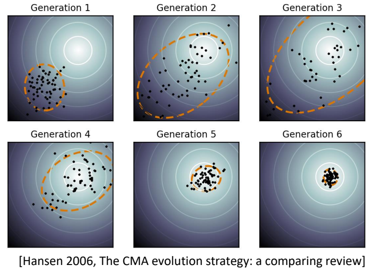
问题:
- 优化虚拟动物的步态
- 目标:行走速度最快
方法:
- 使用 CMA-ES 优化步态参数
- 参数:脚部落点、摆动轨迹、关节角度
结果:
- 自动发现高效的行走模式
- 与真实动物步态相似
实例 2:角色全身轨迹优化 [Al Borno et al. 2013]
问题:
- 优化角色在复杂接触下的轨迹
- 接触序列未知
方法:
- CMA-ES 优化目标轨迹
- 物理仿真评估可行性
优势:
- 无需梯度,处理接触不连续性
- 自动发现合适的接触序列
4.4 与 SAMCON 的关系
CMA-ES 的缺点:
- 每次都从头到尾做仿真,计算量大
- 如果仿真轨迹长,则难收敛
SAMCON 改进:
- 将轨迹分段
- 每段用序列蒙特卡洛方法优化
- 保留多个假设(粒子),避免局部最优
CMA-ES: 整条轨迹 → 一次仿真 → 评估
            ↓
SAMCON: 分段轨迹 → 逐帧仿真 → 粒子滤波
五、CMA-ES 与其他方法对比
5.1 与基于梯度方法对比
| 维度 | CMA-ES | iLQR/DDP |
|---|---|---|
| 梯度需求 | 无需 | 需要(一阶/二阶) |
| 适用问题 | 不可微、非凸 | 平滑、可微 |
| 收敛速度 | 慢(线性) | 快(iLQR 线性,DDP 二阶) |
| 样本效率 | 低(需要大量采样) | 高 |
| 全局性 | 较好(不易陷入局部最优) | 较差(依赖初始猜测) |
| 并行性 | 好(采样可并行) | 较差 |
| 计算成本 | 高(仿真次数多) | 中(需要计算梯度) |
5.2 与其他无梯度方法对比
| 方法 | 适用维度 | 样本效率 | 全局搜索 |
|---|---|---|---|
| CMA-ES | 低~中维 (<100) | 中 | 好 |
| 贝叶斯优化 | 低维 (<20) | 高 | 好 |
| 随机搜索 | 任意 | 低 | 差 |
| 粒子群优化 | 任意 | 中 | 中 |
5.3 方法选择建议
更多方法对比请参见:方法对比与分类。
问题特点 → 推荐方法
─────────────────────────
线性、可微 → LQR
平滑非线性 → iLQR/DDP
接触频繁、不可微 → CMA-ES
样本昂贵 → 贝叶斯优化
高维 (>100) → 考虑基于梯度方法
实时控制 → MPC/SAMCON
需要泛化 → 强化学习 (DeepMimic)
5.4 应用:用 CMA-ES 学习线性反馈策略
除了优化轨迹,CMA-ES 还可以用于学习参数化的策略函数。
问题设定:
- 目标:学习一个反馈策略 \(\pi(s)\),将状态映射到动作
- 参数化:线性策略 \(\delta a = M \cdot \delta s + \hat{a}\)
- 优化变量:反馈矩阵 \(M\) 和前馈项 \(\hat{a}\)
优化流程:
1. 用 SAMCON 优化开环轨迹,得到参考控制 â
2. 参数化线性反馈策略:a = M·δs + â
3. 用 CMA-ES 优化参数 (M, â)
   - 采样候选参数 {θᵢ}
   - 仿真评估每个候选策略
   - 更新高斯分布的均值和方差
4. 输出最优策略参数 θ*
工程实践(Liu et al. 2012 - Terrain Runner):
| 技巧 | 说明 | 效果 |
|---|---|---|
| 手动选择状态 | 仅选择关键状态(根结点旋转、质心位置/速度、支撑脚位置) | 12 维 → 减少无关信息 |
| 手动选择控制 | 仅对少数关键关节加反馈 | 9 维 → 减少优化变量 |
| 矩阵分解 | \(M_{12×9} = M_{12×3} · M_{3×9}\) | 108 参数 → 63 参数 |
优化成本:
- 优化变量:63 维
- 计算时间:12 分钟(24 核并行)
与轨迹优化的对比:
| 轨迹优化 | 策略优化 | |
|---|---|---|
| 输出 | 一条轨迹 \((x,u)\) | 一个策略函数 \(\pi(s)\) |
| 优化对象 | 有限维向量 | 函数参数 \(\theta\) |
| 泛化能力 | ❌ 仅适用于该轨迹 | ✅ 可处理新状态 |
| 计算成本 | 中(秒级) | 高(分钟级) |
✅ 注意:这里的策略优化仍然是离线优化,不同于强化学习的在线学习。
六、工程实践
6.1 调参建议
| 参数 | 推荐值 | 说明 |
|---|---|---|
| \(\lambda\) | \(4 + \lfloor 3 \ln n \rfloor\) | 种群大小 |
| \(\mu\) | \(\lfloor \lambda/2 \rfloor\) | 精英数量 |
| \(\sigma_0\) | 根据问题尺度设置 | 初始步长 |
| \(c_1\) | \(2/n^2\) | 累积学习率 |
| \(c_\mu\) | \(\mu/n^2\) | 精英学习率 |
6.2 实用技巧
1. 参数缩放
- 将参数归一化到 [0, 1] 范围
- 避免某些参数主导搜索
2. 约束处理
- 使用罚函数:\(J' = J + \lambda \cdot \text{constraint}\)
- 或在采样时截断
3. 早停策略
- 如果连续 N 代没有改进,则停止
- 节省计算资源
4. 多起点
- 从多个初始点运行 CMA-ES
- 选择最优结果
6.3 并行化
CMA-ES 的主要计算成本在评估阶段,可以并行:
# 串行(慢)
for i in range(λ):
    f[i] = f(x[i])

# 并行(快)
from joblib import Parallel, delayed
f = Parallel(n_jobs=-1)(delayed(f)(x[i]) for i in range(λ))
七、关键要点总结
核心思想
- 高斯分布建模:将优化变量视为随机变量,用高斯分布表示
- 自适应协方差:根据精英样本更新协方差矩阵,学习搜索方向
- 进化路径:累积历史信息,加速收敛
算法流程
初始化 → 采样 → 评估 → 选择 → 更新 → 检查收敛
   ↑                                        ↓
   └────────────────────────────────────────┘
优缺点
| 优点 | 缺点 |
|---|---|
| 无需梯度,适用于黑盒问题 | 样本效率低,收敛慢 |
| 能处理不可微、非凸问题 | 高维问题效果差 |
| 全局搜索能力强 | 计算成本高 |
| 采样可并行 | 需要调参 |
适用场景
- ✅ 接触频繁的轨迹优化
- ✅ 不可微目标函数
- ✅ 黑盒仿真系统
- ✅ 低~中维优化问题 (<100 维)
- ❌ 实时控制(计算太慢)
- ❌ 高维问题(收敛太慢)
八、深入学习
前置知识
相关方法
参考资料
- Hansen 2006 - The CMA Evolution Strategy: A Comparing Review
- Wampler and Popović 2009 - Optimal Gait and Form for Animal Locomotion
- Al Borno et al. 2013 - Trajectory Optimization for Full-Body Movements with Complex Contacts
代码资源
本文出自 CaterpillarStudyGroup,转载请注明出处。 https://caterpillarstudygroup.github.io/GAMES105_mdbook/
SAMCON(基于采样的运动控制)
✅ 本章定位:理解 序列蒙特卡洛方法 在轨迹优化中的应用,掌握 SAMCON 的核心思想、算法流程以及与 CMA-ES 的对比。
一、从 CMA-ES 到 SAMCON
CMA-ES 的局限性
CMA-ES 是一种强大的无梯度优化方法,但在角色动画中存在以下问题:
| 问题 | 说明 | 影响 |
|---|---|---|
| 全轨迹仿真 | 每次采样需要从头到尾仿真整条轨迹 | 计算量大,效率低 |
| 长轨迹难收敛 | 轨迹越长,搜索空间越大 | 收敛速度慢,容易陷入局部最优 |
| 无法利用时序结构 | 将轨迹视为整体优化 | 忽略了运动的时序依赖性 |
直观理解:
CMA-ES: 采样整条轨迹 → 仿真 100 帧 → 评估
        ↓
        计算成本:100 帧 × λ 个样本 = 100λ 次仿真步
SAMCON 的核心改进
SAMCON (SAmpling-based Motion CONtrol) [Liu et al. 2010, 2015] 针对 CMA-ES 的缺点进行了两项关键改进:
改进 1:分段优化
- 将轨迹分割成多个小段
- 每次只优化一小段,降低搜索空间维度
改进 2:序列蒙特卡洛
- 使用粒子滤波的思想
- 保留多个假设(粒子),避免局部最优
- 逐帧/逐段推进,利用时序结构
SAMCON: 分段采样 → 逐帧仿真 → 粒子滤波
        ↓
        计算成本:每帧 λ 个样本,但收敛更快
二、SAMCON 算法框架
2.1 问题形式化
输入:
- 参考运动片段(Motion Clip):\(M_{\text{ref}} = {m_1, m_2, \dots, m_T}\)
- 初始状态:\(x _0\)
- 物理仿真器
输出:
- 开环控制轨迹:\(u_{0:T}\)
- 物理可行的状态轨迹:\(x_{0:T}\)
目标: $$ \min {u{0:T}} \sum _{t=0}^{T} |x_t - x_t^{\text{ref}}|^2 + \lambda |u_t|^2 $$
s.t. 物理约束(动力学、接触、关节限制等)
2.2 算法流程
算法:SAMCON

输入:
    - 参考运动 M_ref
    - 初始状态 x_0
    - 粒子数量 N
    - 每段长度 L

输出:
    - 控制轨迹 u_{0:T}
    - 状态轨迹 x_{0:T}

1. 初始化粒子集合 P_0 = {x_0}

2. For t = 0 to T-1:

   (a) 采样阶段
       对每个粒子 x_t^(i) ∈ P_t:
           采样偏移量 δ ~ N(0, Σ)
           生成候选控制 u_t^(i) = u_ref(t) + δ

   (b) 仿真阶段
       对每个候选控制 u_t^(i):
           用物理仿真器仿真一帧
           得到新状态 x_{t+1}^(i)

   (c) 评估阶段
       计算每个新状态的得分:
       score^(i) = -||x_{t+1}^(i) - x_{t+1}^ref||²

   (d) 选择阶段
       根据得分对粒子排序
       保留前 N 个最优粒子
       P_{t+1} = {top-N particles}

   (e) 重采样(可选)
       如果粒子多样性过低:
           对优质粒子进行重采样

3. 从最终粒子集合中提取最优轨迹
2.3 可视化理解
时刻 t: 粒子集合 P_t
  o  o  o     o = 粒子(假设)
    o   o
  o      o
        ↓ 采样 + 仿真
时刻 t+1: 新粒子集合
      o  o o    o = 优质粒子(保留)
    o  o× ××    × = 劣质粒子(淘汰)
      o  ×
        ↓ 选择
时刻 t+1: 筛选后
      o  o o    保留 N 个最优
    o  o
三、SAMCON 关键技术
3.1 偏移量采样
核心思想:在参考轨迹上添加随机偏移,跟踪偏移后的轨迹。
$$ u_t^{(i)} = u_{\text{ref}}(t) + \delta^{(i)}, \quad \delta^{(i)} \sim \mathcal{N}(0, \Sigma) $$
采样策略:
| 策略 | 说明 | 适用场景 |
|---|---|---|
| 高斯采样 | \(\delta \sim \mathcal{N}(0, \Sigma)\) | 一般情况 |
| 自适应方差 | 根据上一帧结果调整 \(\Sigma\) | 动态环境 |
| 重要性采样 | 偏向更有希望的区域 | 复杂约束 |
3.2 粒子选择
选择标准: $$ \text{score}^{(i)} = -|x_{t+1}^{(i)} - x_{t+1}^{\text{ref}}|^2 - \lambda |u_t^{(i)}|^2 $$
选择策略:
| 策略 | 说明 | 优点 | 缺点 |
|---|---|---|---|
| Top-N | 保留得分最高的 N 个 | 简单高效 | 可能丢失多样性 |
| 轮盘赌 | 按得分比例概率选择 | 保持多样性 | 收敛稍慢 |
| 精英保留 | 最优粒子直接晋级 + 随机选择 | 兼顾收敛与多样性 | 需要调参 |
3.3 重采样机制
问题:经过多轮选择后,粒子可能趋于一致(粒子退化)
解决:定期重采样,补充多样性
重采样条件:
- 粒子多样性低于阈值
- 连续 k 帧没有改进
- 检测到陷入局部最优

重采样方法:
1. 对优质粒子添加高斯噪声
2. 从历史优质粒子中随机复制
3. 完全重新采样(探索模式)
3.4 分段策略
分段方式:
| 方式 | 说明 | 适用场景 |
|---|---|---|
| 固定长度 | 每 L 帧一段 | 均匀运动 |
| 按关键帧 | 在接触事件处分段 | 步态、跳跃等 |
| 自适应 | 根据误差动态调整 | 复杂运动 |
段间衔接:
- 保证状态连续性(位置、速度)
- 使用重叠窗口平滑过渡
四、SAMCON 与相关方法对比
4.1 与 CMA-ES 对比
| 维度 | CMA-ES | SAMCON |
|---|---|---|
| 优化单位 | 整条轨迹 | 分段/逐帧 |
| 搜索空间 | 高维(T × 控制维度) | 低维(每段控制维度) |
| 仿真成本 | 全轨迹仿真 | 单帧/单段仿真 |
| 收敛速度 | 慢(尤其长轨迹) | 快(分段降低难度) |
| 抗局部最优 | 中(依赖协方差自适应) | 高(粒子多样性) |
| 内存需求 | 低 | 中(需存储粒子集合) |
| 并行性 | 好(样本独立) | 中(帧间依赖) |
4.2 与 MPC 对比
| 维度 | SAMCON | MPC |
|---|---|---|
| 优化方法 | 序列蒙特卡洛(采样) | 数值优化/解析 |
| 梯度需求 | 无需 | 通常需要 |
| 适用问题 | 不可微、接触频繁 | 平滑、可微 |
| 计算成本 | 中(大量仿真) | 高(求解优化问题) |
| 实时性 | 中(可增量计算) | 低(需要完整求解) |
| 鲁棒性 | 高(粒子多样性) | 中(依赖初始猜测) |
4.3 方法选择建议
更多方法对比请参见:方法对比与分类。
应用场景 → 推荐方法
─────────────────────────
离线轨迹优化,平滑问题 → iLQR/DDP
离线轨迹优化,接触频繁 → CMA-ES
在线实时控制,简单场景 → SAMCON
在线实时控制,复杂场景 → MPC
需要泛化能力 → DeepMimic/强化学习
五、SAMCON 的应用实例
5.1 运动跟踪 [Liu et al. 2010]
问题:
- 输入:动捕数据(Motion Capture)
- 目标:生成物理可行的跟踪轨迹
- 挑战:动捕数据可能不满足物理约束(穿地、失衡等)
方法:
- 用动捕数据作为参考轨迹 \(M_{\text{ref}}\)
- SAMCON 逐帧采样偏移量
- 物理仿真验证可行性
- 选择最接近参考的粒子
结果:
- 自动修正穿地问题
- 维持动态平衡
- 保持原始运动风格
5.2 地形自适应行走
问题:
- 在不平坦地形上行走
- 需要调整步态适应地形
SAMCON 方案:
每帧:
  1. 采样多种落脚点
  2. 仿真验证稳定性
  3. 选择最优落脚点
  4. 继续推进
优势:
- 无需预先规划接触序列
- 自动适应未知地形
- 实时响应扰动
5.3 跌倒恢复
问题:
- 角色受到外力推击
- 需要快速恢复平衡
SAMCON 方案:
- 增大采样方差(探索模式)
- 增加粒子数量
- 以稳定性为首要评分标准
结果:
- 自动跨步恢复平衡
- 必要时主动倒地
- 倒地后自主爬起
六、工程实践
6.1 参数设置
| 参数 | 推荐值 | 说明 |
|---|---|---|
| 粒子数量 N | 50-200 | 越多效果越好,但计算成本增加 |
| 采样方差 \(\Sigma\) | 根据任务调整 | 大→探索,小→开发 |
| 段长度 L | 5-20 帧 | 根据运动类型调整 |
| 精英比例 | 10-30% | 保留优质粒子 |
6.2 实用技巧
1. 自适应方差
if diversity < threshold:
    Σ *= 1.5  # 增加探索
elif convergence_speed > target:
    Σ *= 0.8  # 加快收敛
2. 粒子多样性度量 $$ \text{diversity} = \frac{1}{N^2} \sum_{i,j} |x^{(i)} - x^{(j)}| $$
3. 渐进式优化
- 先用少量粒子快速得到可行解
- 再用更多粒子精细化
4. 缓存与重用
- 缓存仿真结果
- 重用历史优质粒子
6.3 性能优化
并行化:
# 粒子仿真可并行
from joblib import Parallel, delayed

def simulate_particle(particle):
    # 仿真一帧
    return new_state

new_states = Parallel(n_jobs=-1)(
    delayed(simulate_particle)(p) for p in particles
)
向量化:
- 将粒子状态组织成数组
- 使用 SIMD/GPU 加速仿真
七、关键要点总结
核心思想
- 分段优化:将长轨迹分割为小段,降低搜索空间维度
- 序列蒙特卡洛:使用粒子滤波思想,保留多个假设
- 逐帧推进:利用时序结构, incremental 构建完整轨迹
算法流程
初始化 → 采样偏移 → 物理仿真 → 评估选择 → 重采样 → 推进到下一帧
优缺点
| 优点 | 缺点 |
|---|---|
| 无需梯度,适用于黑盒问题 | 需要大量仿真 |
| 分段优化,收敛快 | 粒子退化问题 |
| 粒子多样性,抗局部最优 | 需要调参 |
| 可实时应用 | 高维问题效果差 |
适用场景
- ✅ 运动跟踪(动捕数据物理化)
- ✅ 地形自适应行走
- ✅ 跌倒恢复与平衡控制
- ✅ 在线实时控制
- ❌ 离线全局优化(用 CMA-ES 更合适)
- ❌ 高维精细优化(用 iLQR 更合适)
八、深入学习
前置知识
相关方法
参考资料
- Liu et al. 2010 - Sampling-based Motion Control
- Liu et al. 2015 - Terrain Runner
- Al Borno et al. 2013 - Trajectory Optimization for Full-Body Movements
代码资源
- MOCCA - Motion Control and Optimization - UBC 的运动控制库
本文出自 CaterpillarStudyGroup,转载请注明出处。 https://caterpillarstudygroup.github.io/GAMES105_mdbook/
六、优化方法分类概览
轨迹优化方法可以从多个维度进行分类,详细的对比和分类请参见:方法对比与分类。
简要总结:
| 维度 | 分类 | 代表方法 |
|---|---|---|
| 优化时机 | 离线 vs. 在线 | CMA-ES/iLQR/DDP vs. MPC/SAMCON |
| 求解方法 | 解析法 vs. 数值法 vs. 学习法 | LQR vs. iLQR/DDP/CMA-ES vs. DeepMimic/AMP |
| 梯度需求 | 基于梯度 vs. 无梯度 | iLQR/DDP vs. CMA-ES/SAMCON |
七、与 DeepMimic/AMP 的关系
| 维度 | 轨迹优化 | DeepMimic/AMP |
|---|---|---|
| 输出 | 单一轨迹 \(\mathbf{x}_{0:T}\) | 策略 \(\pi(\mathbf{a} |
| 计算时机 | 离线优化(每任务一次) | 训练一次,在线推理 |
| 泛化能力 | 无(仅适用于该轨迹) | 有(可处理新情况) |
| 计算成本 | 高(分钟级) | 低(毫秒级推理) |
| 适用场景 | 特定动作生成 | 通用角色控制 |
关系:
- 轨迹优化结果可作为 RL 的参考轨迹
- RL 可学习模仿轨迹优化的行为
八、关键要点总结
-
优化变量:状态轨迹 \(\mathbf{x}{0:T}\) + 控制轨迹 \(\mathbf{u}{0:T-1}\)
-
目标函数:
- 终端代价 \(J_T(\mathbf{x}_T)\)
- 运行代价 \(\sum J_t(\mathbf{x}_t, \mathbf{u}_t)\)
- 常见项:跟踪误差、控制 effort、平滑项
-
约束条件:
- 动力学约束(运动方程)
- 接触约束(不穿透、摩擦锥)
- 控制/状态限制
-
方法选择建议:
- 线性系统 → LQR
- 平滑非线性 → iLQR/DDP
- 接触频繁/不可微 → CMA-ES
- 实时控制 → MPC/SAMCON
- 需要泛化 → DeepMimic/AMP
📚 深入学习:
P3
Recap
| feedforward | feedback |
|---|---|
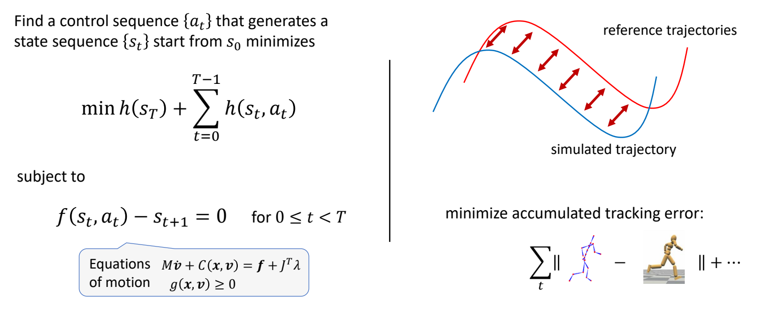 |  |
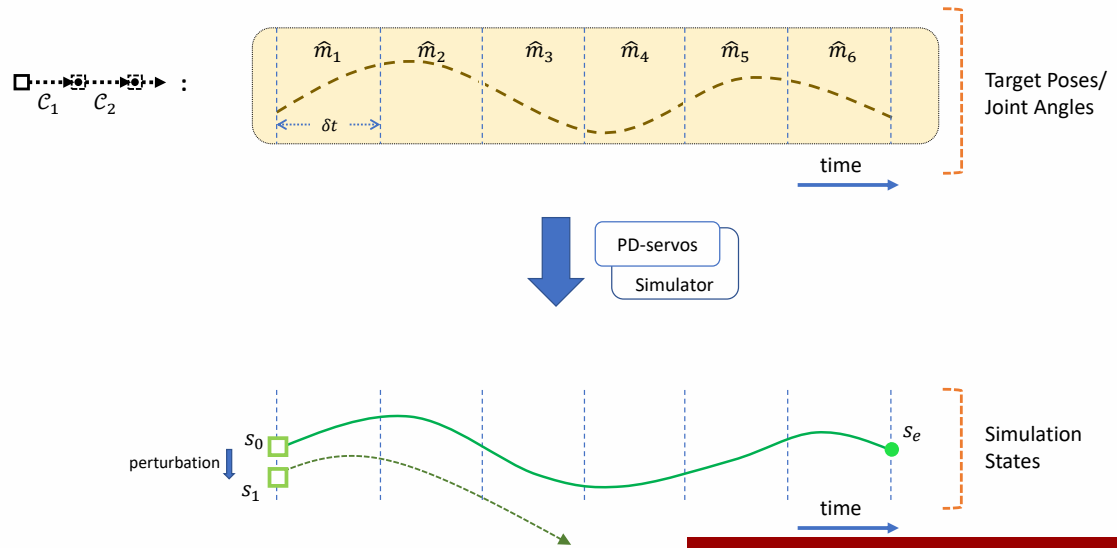 | 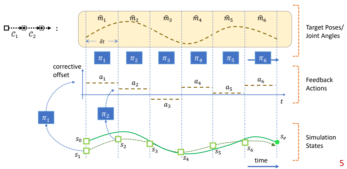 |
✅ 开环控制:只考虑初始状态。 ✅ 前馈控制:考虑初始状态和干挠。 ✅ 前馈控制优化的是轨迹。 ✅ 反馈控制优化的是控制策略,控制策略是一个函数,根据当前状态优化轨迹。
P9
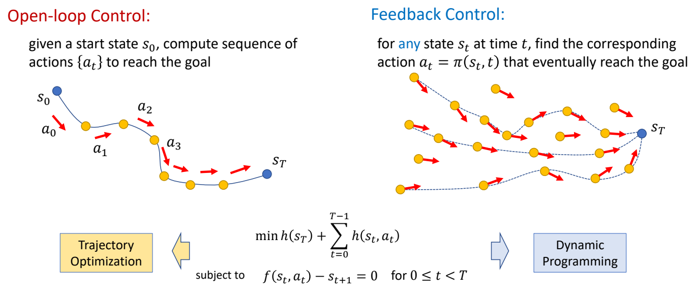
✅ Feedback 类似构造一个场,把任何状态推到目标状态。
P10
开环控制
问题描述
$$ \begin{matrix} \min_{x} f(x)\ 𝑠.𝑡. g(x)=0 \end{matrix} $$

P12
把硬约束转化为软约束
$$ \min_{x} f(x)+ wg(x) $$
(^*) The solution (x^\ast) may not satisfy the constraint
P16
Lagrange Multiplier - 把约束条件转化为优化
✅ 拉格朗日乘子法。
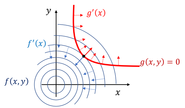
✅ 通过观察可知,极值点位于({f}'(x)) 与 (g) 的切线垂直,即 ({f}' (x)) 与 ({g}' (x)) 平行。(充分非必要条件。)
因此:
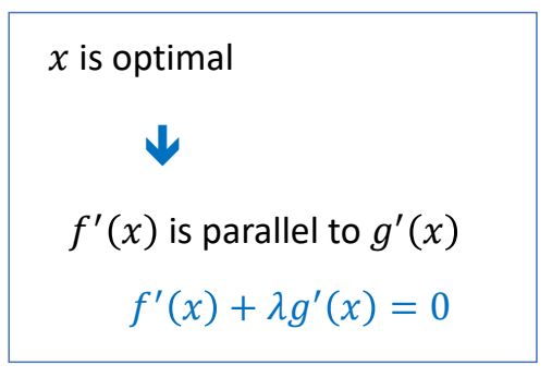
Lagrange function
$$ L(x,\lambda )=f(x)+\lambda ^Tg(x) $$
✅ 把约束条件转化为优化。
P18
Lagrange Multiplier
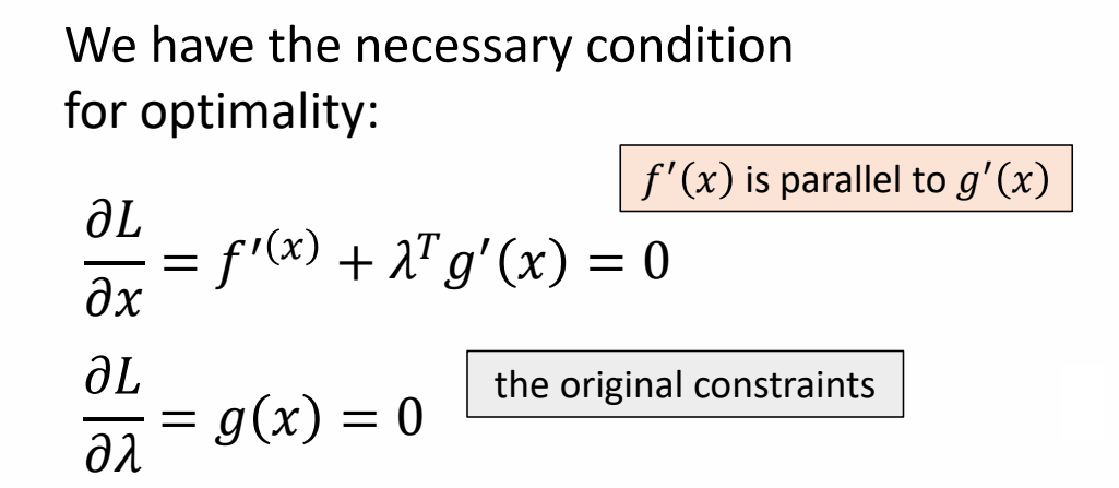
✅ 这是一个优化问题,通过梯度下降找到极值点。
P20
Solving Trajectory Optimization Problem
定义带约束的优化问题
Find a control sequence {(a_t)} that generates a state sequence {(s_t)} start from (s_o) minimizes
$$ \min h (s_r)+\sum _{t=0}^{T-1} h(s_t,a_t) $$
✅ 因为把时间离散化,此处用求和不用积分。
subject to
$$ \begin{matrix} f(s_t,a_t)-s_{t+1}=0\ \text{ for } 0 \le t < T \end{matrix} $$
✅ 运动学方程,作为约束
转化为优化问题
The Lagrange function
$$ L(s,a,\lambda ) = h(s _ T)+ \sum _ {t=0} ^ {T-1} h(s _t,a _t) + \lambda _ {t+1}^T(f(s _t,a _t) - s _ {t+1}) $$
P27
求解拉格朗日方程
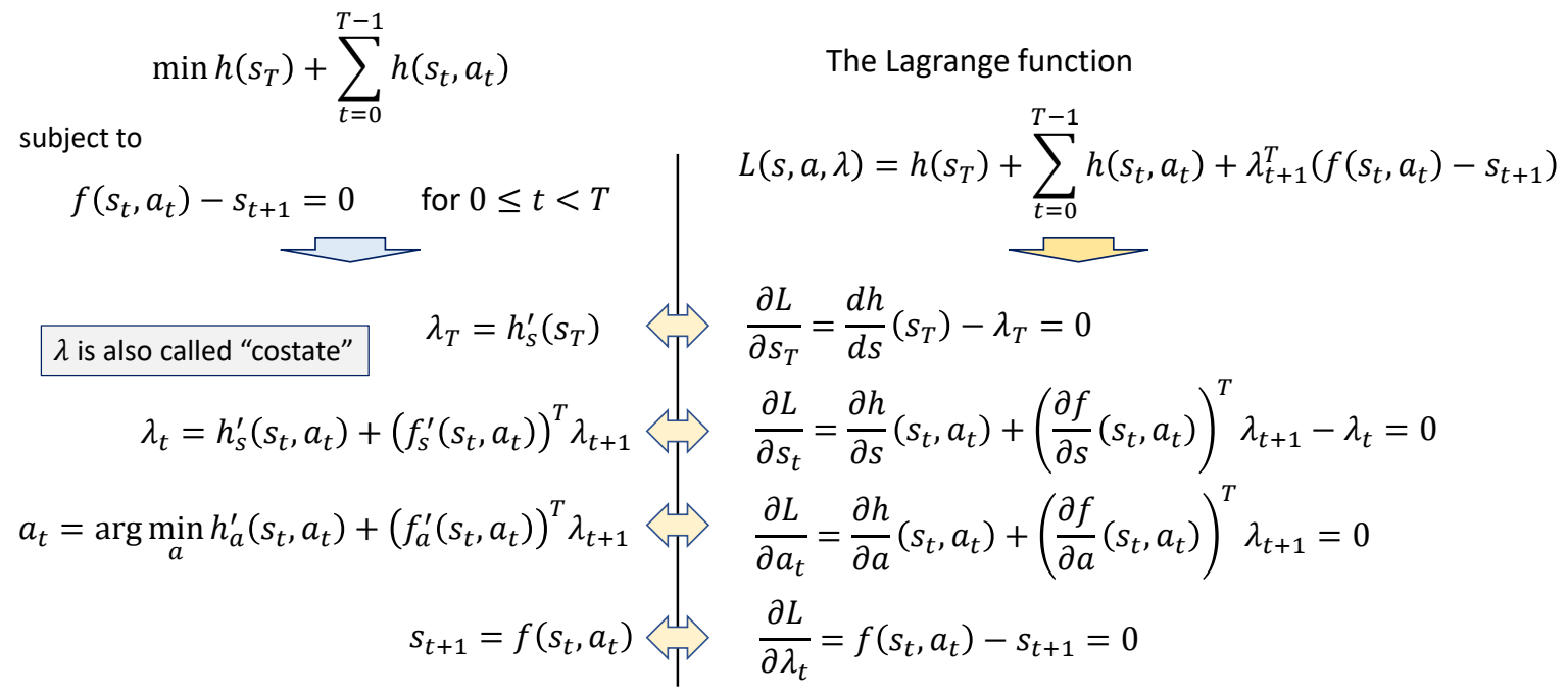
✅ 拉格朗日方程,对每个变量求导,并令导数为零。因此得到右边方程组。 ✅ 右边方程组进一步整理,得到左边。 ✅ (\lambda ) 类似于逆向仿真。 ✅ 公式 3:通过转为优化问题求 (a).
P30
Pontryagin's Maximum Principle for discrete systems
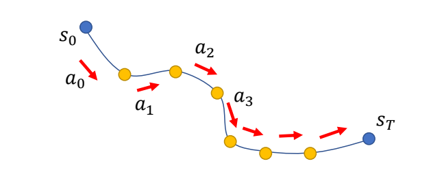
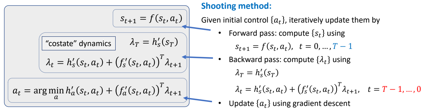
✅ 方程组整理得到左边,称为 PMP 条件。是开环控制最优的必要条件。
P32
Optimal Control
Open-loop Control: given a start state (s_0), compute sequence of actions {(a_t)} to reach the goal
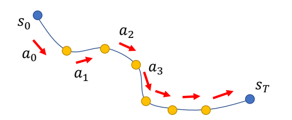
Shooting method directly applies PMP. However, it does not scale well to complicated problems such as motion control… (
) Need to be combined with collocation method, multiple shooting, etc. for those problems. (
) Or use derivative-free approaches.
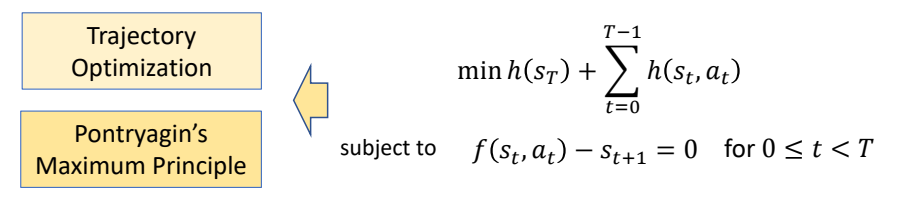
✅ 对于复杂函数,表现比较差,还需要借助其它方法。
闭环控制
P34 P49
The Bellman Equation
Mathematically, an optimal value function (V(s)) can be defined recursively as:
$$ V(s)=\min_{a} (h(s,a)+V(f(s,a))) $$
✅ h 代表 s 状态下执行一步 a 的代价。f 代表 s 状态下执行一步 a 之后的状态。
If we know this value function, the optimal policy can be computed as
$$ \pi (s)=\arg \min_{a} (h(s,a)+V(f(s,a))) $$
✅ pi 代表一种策略,根据当前状态 s 找到最优的下一步 a。 ✅ This arg max can be easily computed for discrete control problems. But there are not always closed-forms solution for continuous control problems.
or
$$ \begin{matrix} \pi (s)=\arg \min_{a} Q(s,a)\ \text{where} \quad \quad Q(s,a)=h(s,a)+V(f(s,a)) \end{matrix} $$
Q-function 称为 State-action value function Learning (V(s)) and/or (Q(s,a)) is the core of optimal control / reinforcement learning methods
✅ 强化学习最主要的目的是学习 (V) 函数和 (Q) 函数,如果 (a) 是有限状态,遍历即可。但在角色动画里,(a) 是连续状态。
动态规划推导(逆向归纳法)
✅ 由于存在最优子结构(optimal substructure),可以从最后一步往前推导:
- 每一步只需要考虑从当前状态到终点的最优解
- 最后一个状态的 Value 计算与 \(a\) 无关
- 计算完最后一步,再计算倒数第二步,依次往前推
Value Function 的形式
假设从时刻 \(t\) 到终点的最优代价(Value Function)具有二次形式:
$$ V _t(s) = s ^T P _t s $$
其中 \(P _t\) 是对称矩阵。
本文出自 CaterpillarStudyGroup,转载请注明出处。
https://caterpillarstudygroup.github.io/GAMES105_mdbook/
P33
简化问题分析
✅ 仍以方块移动到目标高度为例。
问题描述
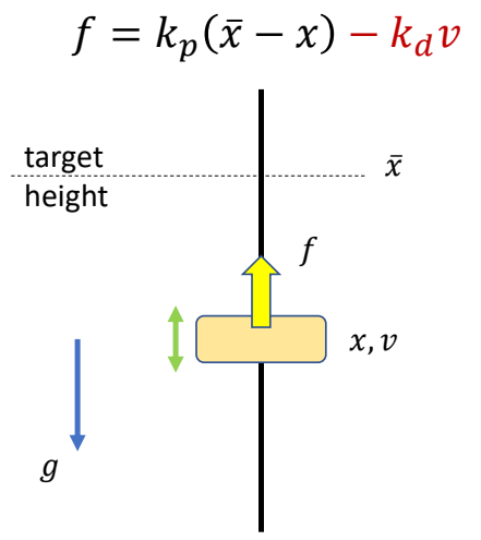
Compute a target trajectory \(\tilde{x} (t)\) such that the simulated trajectory \(x(t)\) is a sine curve.
目标函数
$$ \min_ {(x_n,v_n,\tilde {x} _n)} \sum _ {n=0}^{N} (\sin (t_n)-x_n)^2+\sum _ {n=0}^{N} \tilde {x}^2_n $$
✅ 目标函数:目标项+正则项
约束
$$ \begin{align*} s.t. \quad & v _ {n+1}= v_ n+h (k _ p( \tilde {x} _n-x_n)-k _ dv_n) \\ & v _ {n+1} = x _ n + hv _ {n+1} \end{align*} $$
✅ 约束:半隐式积分的运动方程
P34
| Hard constraints: | 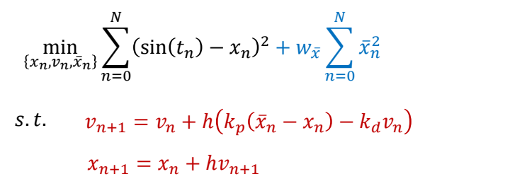 |
| Soft constraints: | 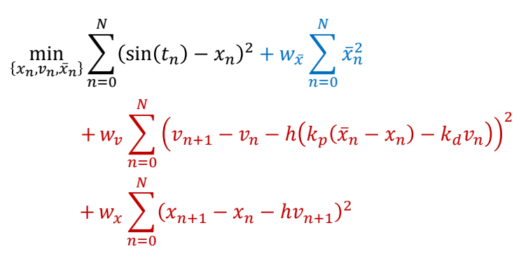 |
✅ 以两种方式体现约束:
✅(1)Hard:必须满足,难解,不稳定。
✅(2)Soft:尽可能满足,易求解。
P35
参数简化
Collocation methods:
Assume the optimization variables {\(x_n, v_n, \tilde{x}_n\)} are values of a set of parametric curves
- typically polynomials or splines
Optimize the parameters of the curves \(\theta\) instead
- with smaller number of variables than the original problem
✅ 要优化的参数量太大,难以优化。
✅ 解决方法:假设参数符合特定的曲线,只学习曲线的参数,再生成完整的参数。
P37
优化方法
How to solve this optimization problem?
Gradient-based approaches:
- Gradient descent
- Newton’s methods
- Quasi-Newton methods
- ……
P39
Trajectory Optimization for Tracking Control
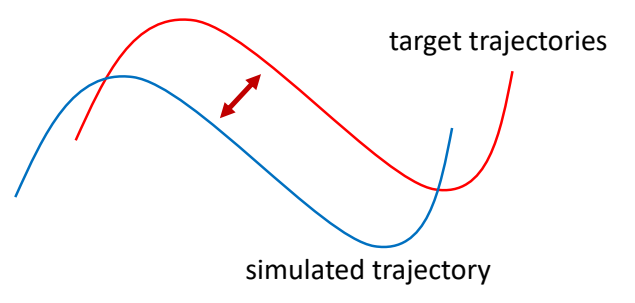
find a target trajectory
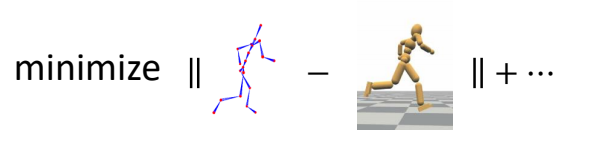
✅ 把动捕结果当成初始解,然后以优化的方式找到合理轨迹。
P40
Problem with Gradient-Based Methods
- The optimization problem is usually highly nonlinear, gradients are unreliable
- The system is a black box with unknow dynamics, gradients are not available
解决方法: Derivative-Free Optimization
-
Iterative methods
- Goal: find the variables 𝒙 that optimize \(f(x)\)
- Determining an initial guess of \(x\)
- Repeat:
- Propose a set of candidate variables {\(x_i\)} according to \(x\)
- Evaluate the objective function \(f_i=f(x_i)\)
- Update the estimation for \(x\)
-
Examples:
- Bayesian optimization, Evolution strategies (e.g. CMA-ES), Stochastic optimization, Sequential Monte Carlo methods, ……
✅ 启发式方法或随机采样方法,不需要梯度。
✅ 缺点:慢、不精确。
P43
CMA-ES
- Covariance matrix adaptation evolution strategy (CMA-ES)
- A widely adopted derivative-free method in character animation
Goal: find the variables 𝒙 that optimize \(f(x)\)
- Initialize Gaussian distribution \(x\sim \mathcal{N} (\mu ,\Sigma )\)
- Repeat:
- sample candidate variables {\(x_i\)} \( \sim \mathcal{N} (\mu ,\Sigma )\)
- Evaluate the objective function \(f_i=f(x_i)\)
- Involve simulation and generate simulation trajectories
- Sort {\(f_i\)} and keep the top \(N\) elite samples
- Update \(\mu ,\Sigma \) according to the elite samples
✅ 优点:稳定,无梯度,可用于黑盒系统。
P44
🔎 [Wampler and Popović 2009 - Optimal Gait and Form for Animal Locomotion]
P45
✅ [Al Borno et al. 2013 - Trajectory Optimization for Full-Body Movements with Complex Contacts]
✅ 只优化目标轨迹,不优化仿真轨迹。因为仿真轨迹可以通仿真得到。
P46
SAMCON
✅ CMA-ES 的缺点:
(1)每次都从头到尾做仿真,计算量大。
(2)如果仿真轨迹长,则难收敛。
✅ 改进方法:每次采样,只考虑下面一帧。
🔎 SAmpling-based Motion CONtrol [Liu et al. 2010, 2015]
- Motion Clip → Open-loop control trajectory
- A sequential Monte-Carlo method
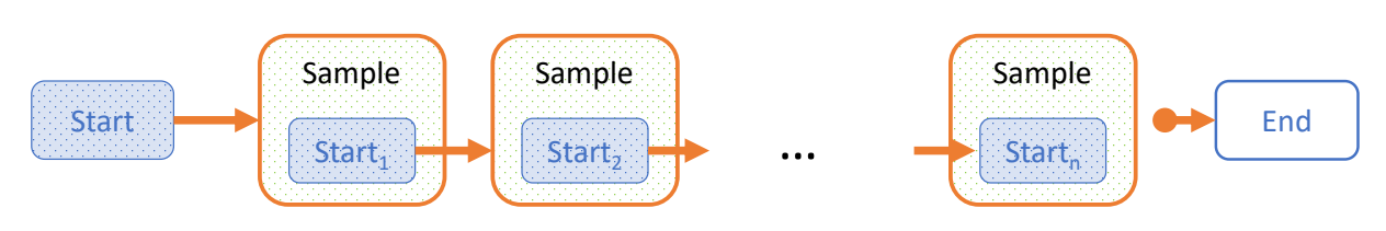
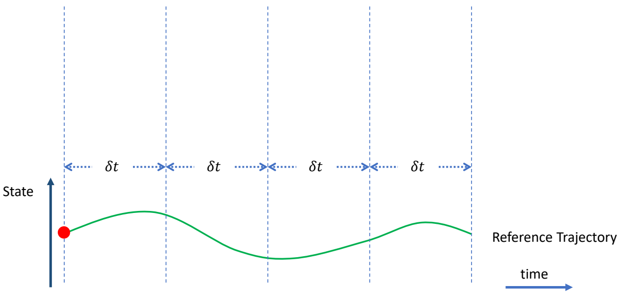 | ✅ 把轨迹分割开,每次优化一小段。 |
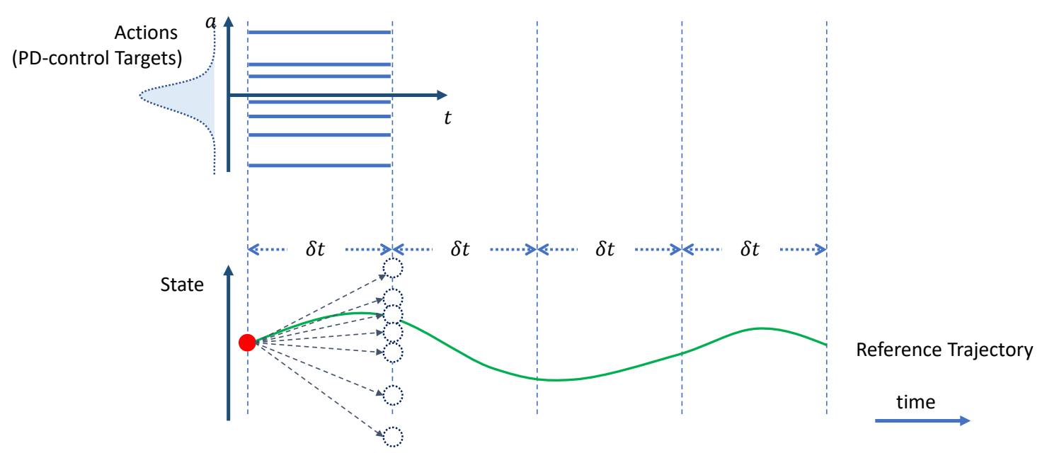 | ✅ 在目标轨迹上增加偏移,跟踪偏移之后的轨迹。 ✅ 偏移量未知,因此以高斯分布对偏移量采样。 ✅ 高斯分布可由其它分布代替。 |
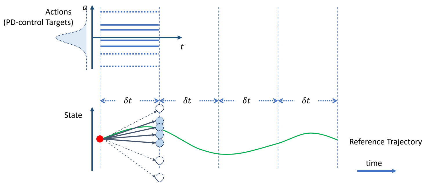 | ✅ 对每个偏移量做一次仿真,生成新的状态,保留其中与当目标接近的 N 个。 |
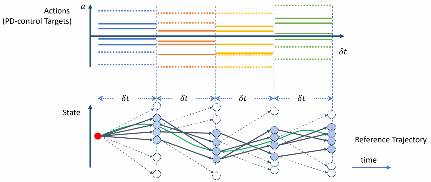 | ✅ 从上一步 N 个中随机选择出发点,以及随机的偏移量,再做仿真与筛选。 |
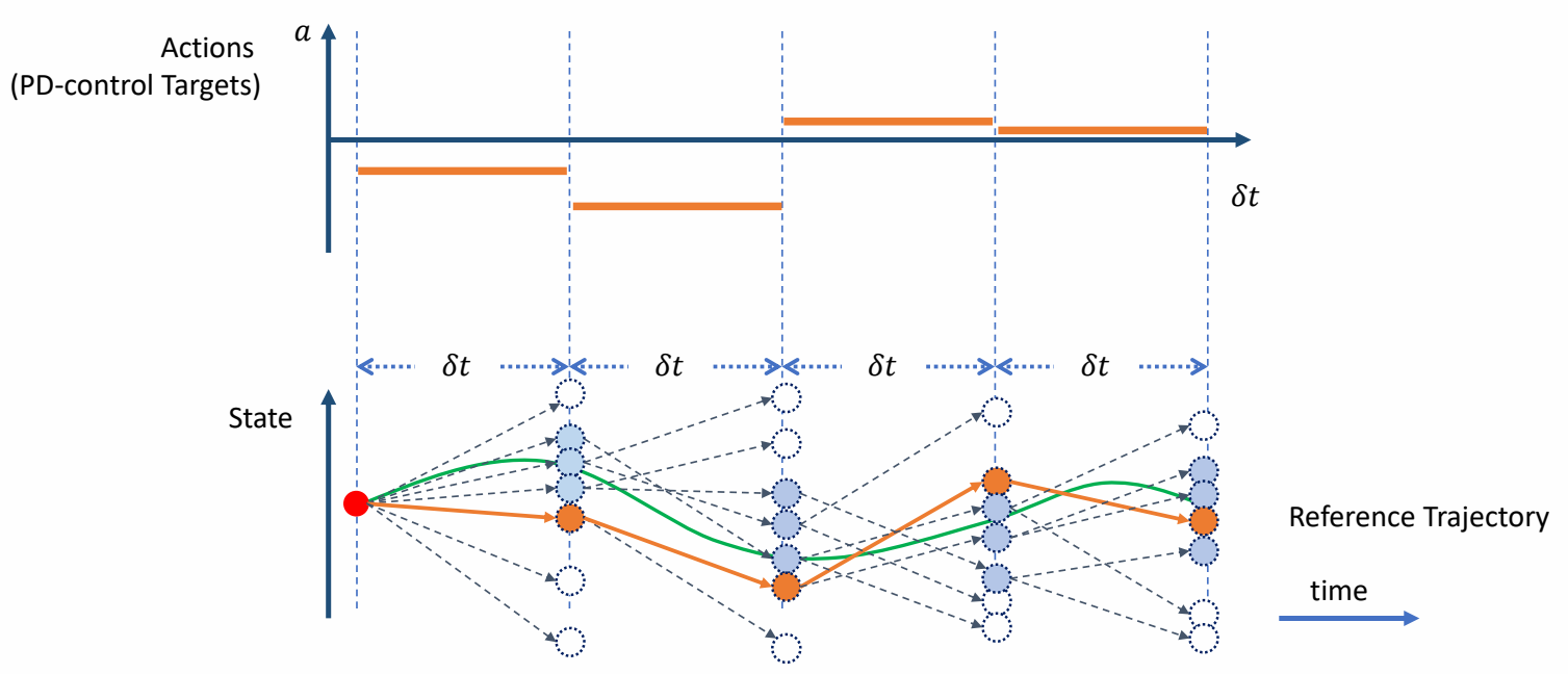 | ✅ 最终找到一组最接近的。 ✅ 原理:只选一个容易掉入局部最优,因此保留多个。 ✅ 蒙特卡罗+动态规划 |
✅ 优点:穿膜问题也能被修正掉,可还原动捕数据,可根据环境影响而自动调整。
P54
Feedforward & Feedback Control
Feedforward Control
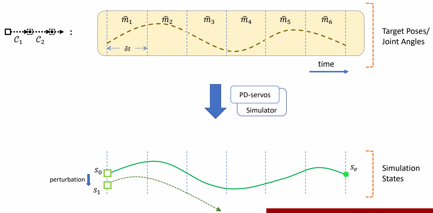
✅ 前馈控制,要求每一步的起始状态都是在获取轨迹过程中能得到的状态。
✅ 如果对起始状态加一点挠动,状态会偏离很远。
P56
Feedback Control
✅ 解决方法:引入反馈策略。根据当前偏差,自动计算出更正,把更正叠加到控制轨迹上。
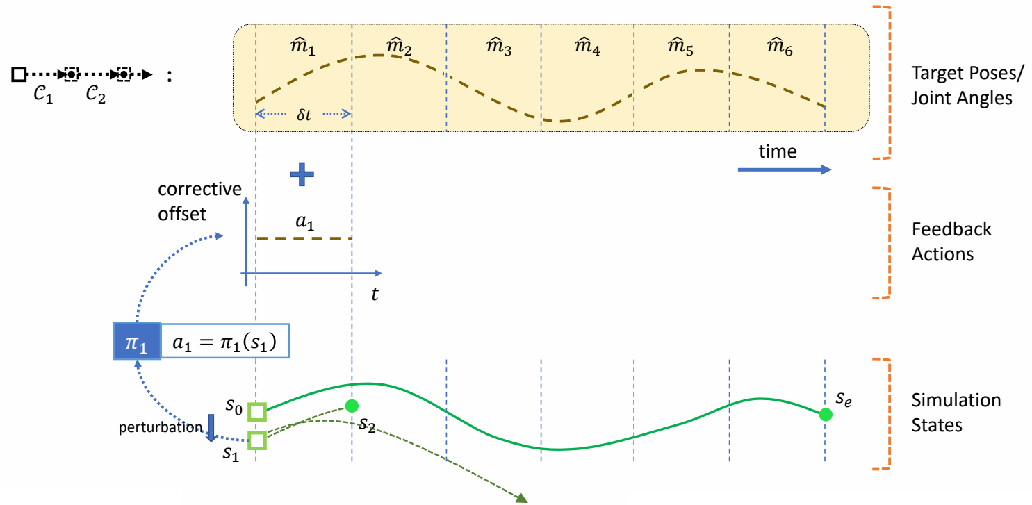 |
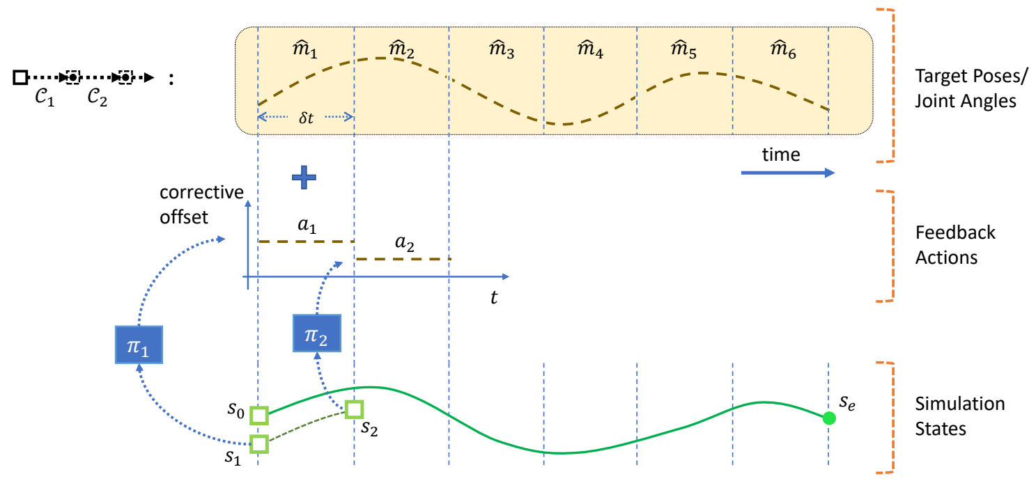 |
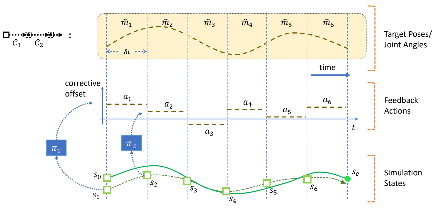 |
P101
What’s Next?
Digital Cerebellum
Large Pretrained Model for Motion Control
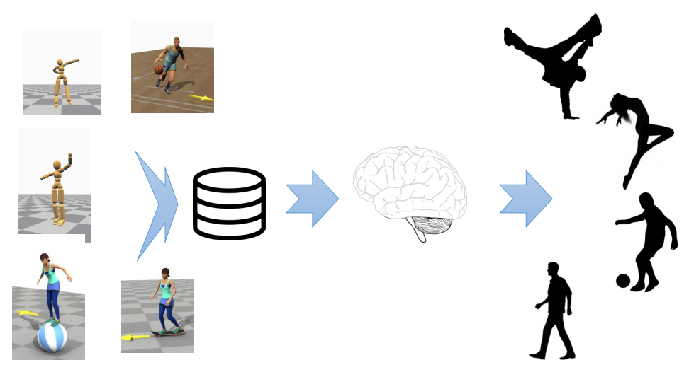
P102
Cross-modality Generation
- \(\Leftrightarrow\) LLM \(\Leftrightarrow\) Text/Audio \(\Leftrightarrow\) Motion/Control \(\Leftrightarrow\) Image/Video \(\Leftrightarrow\)
- Digital Actor?
本文出自CaterpillarStudyGroup,转载请注明出处。
https://caterpillarstudygroup.github.io/GAMES105_mdbook/
强化学习在角色动画中的应用
强化学习适用于在给定极少且不确定的未来信息的情况做出当前的最优决策。
在角色动画领域中,强化学习有两种使用场景:
- 高层控制:根据任务目标规划任务的执行方案。执行方案可能是明确的动画轨迹,也可能是latent code,或者是其它控制信号。
- 中层控制:根据角色当前的状态,规划自己的动作,保证能完成高层给的执行方案且保证较好的动作质量。在动力学方法中,『较好的动作质量』即不摔倒,走得稳。在运动学方法中,『较好的动作质量』指动作转移合理。
高层控制和中层控制都适合用强化学习解决,但也可以通过其它方法解决。通过梳理相关工作,分为以下几类:
- 把高层控制和中层控制看作是一个端到端的任务,用一个强化学习同时解决『执行方案』和『执行细节』两个问题。
- 分别解决高层控制和中层控制,各自使用一个强化学习。
- 高层控制使用强化学习来解决,中层控制使用其它方法。例如运动学方法使用运动转移先验模型。动力学方法可以使用轨迹优化(如果高层输出的是轨迹)方法或者直接使用前向推理方向。
- 中层使用强化学习来解决『走得好』的问题,高层则通过其它方法生成执行方案。例如生成类的方法、Motion Matching或者直接使用动捕数据。
- 也可以完成不用强化学习。直接端到端地生成动作,或者分别用不同的方法解决两个level的控制问题。这一类方法不在本页的讨论范围中。
关于参考动作,有没有参考动作对结果影响非常大。参考动作主要有三个作用:
- 加速训练收敛
- 让动作更『人』
- 定义动作的风格
参考动作发挥作用的方法主要有三种:
- GT,直接作为模型的模仿目标
- 鉴定,用于判断生成动作与参考动作是否相似
- 提取数据的关节特征,构造模型的目标函数
除了参考动作,还有其它构造数据的方式:
- 对参考动作做增强
- 用传统算法构造数据
- 从生成的动作中挑一些好的
mindmap
强化学习在角色动画中的应用
    端到端方案
        端到端 RL
            在线 RL
            离线 RL
    分层控制方案
        DL + DL
        DL + 非 DL
        非 DL + DL
        非 DL + 非 DL
端到端的强化学习方案
在线RL
| 方法 | 状态空间 S | 动作空间 A | 奖励函数 R | 核心贡献 |
|---|---|---|---|---|
| Feature-Based2010 | 物理特征(角动量等) | 关节力矩 | 手工设计多目标 | 高层特征控制器 |
| Nerve Net2015 | 关节 + 根节点状态 | 关节力矩 | 任务奖励 | 通用多角色控制器 |
| Predict-and-Simulate2019 | 状态 + 目标 | PD 目标 | 任务奖励 | 从无组织数据学习 |
| Gait-Conditioned Reinforcement Learning with Multi-Phase Curriculum for Humanoid Locomotion2025 | 关节 +IMU+ 命令 | PD 目标轨迹 | 步态条件奖励 (独热路由) | PPO+RNN |
离线RL
由于RL模型只能针对特定任务训练,所以有些方法会离线训练多个RL模型,再用非RL蒸馏出一个同样功能的非RL模型供在线使用。
| 方法 | 状态空间 S | 动作空间 A | 训练范式 | 蒸馏源 |
|---|---|---|---|---|
| DiffuseLoco2024 | 关节 + 根节点 + 技能标签 | 31D PD 目标 | 纯离线 | 多专家 RL |
| PDP2024 | 物理状态 + 任务标签 | 多帧 PD 目标 | 离线 BC | 多任务 RL 专家 |
| 维度 | DiffuseLoco | PDP |
|---|---|---|
| 数据源 | 闭环离线 RL 数据 | RL 专家轨迹 |
| 模型类型 | 扩散 | 扩散 |
| 输出 | 单帧 PD 目标 | 多帧序列 |
| 物理稳定 | ✅ RL 专家保证 | ✅ RL 专家保证 |
DL + DL
| 方法 | 状态空间 S | 动作空间 A | 奖励函数 R | 价值函数 V | 算法 |
|---|---|---|---|---|---|
| DeepLoco (2017) | LLC: 110D (关节 + 根节点 + 相位) | LLC: 22D 关节 PD 目标 | LLC: 姿势风格 + 末端位置 + 速度 + 平衡 | CACLA Critic | Actor-Critic+CACLA |
| HLC: 1129D (+32×32 地形图) | HLC: 5D 步法计划 | HLC: 朝目标方向移动 | CACLA Critic | Actor-Critic+CACLA | |
| ASE (2022) | 120D 身体配置 + 技能 z | 低级: 31D PD 目标 | 对抗奖励 + 技能多样性奖励 | PPO Critic | PPO + 互信息最大化 |
| 120D 身体配置 + 任务目标 | 高级: z̄→z (球面) | 任务奖励 + 风格奖励 | PPO Critic | PPO + 互信息最大化 |
非DL + DL
| 方法 | 上层方法及输出 | 状态空间 S | 动作空间 A | 奖励函数 R | 价值函数 V | 算法 |
|---|---|---|---|---|---|---|
| DeepMimic (2018) | 固定轨迹 (Mocap 时间序列) | 关节 [p,v,q,ω] + 相位 φ | PD 目标 | 模仿奖励 + 任务奖励 模仿奖励=姿势 + 速度 + 末端 + 质心 | PPO Critic GAE(λ) | PPO |
| DReCon2019 | MM动态生成轨迹 | 角色状态 + 辅助信息 +MM 参考 | PD 目标 | 跟踪奖励 + 稳定性奖励 | PPO Critic | PPO+MM |
| AMP (2021) | Mocap轨迹 | ~120D 躯干 + 关节 + 末端 | ~31D 关节目标旋转 | 任务奖励 + 风格奖励 风格奖励由判别器给出 | PPO Critic | PPO+LS-GAN |
| ControlVAE2023 | CVAE输出z | 120D 身体配置 | 31D PD 目标 | 任务奖励 + VAE 重建奖励 | PPO Critic | VAE+PPO |
| CLOSD2025 | 扩散规划输出轨迹 | 角色状态 + 辅助信息 | PD 控制器目标 | 文本 + 目标双条件 | PPO Critic | 扩散规划 + RL 跟踪 |
| DARTControl2025 | Latent Diffusion输出z | 动作历史 + 文本 + 空间目标 | Latent noise optimization | 空间目标达成度 + 动作质量 | PPO Critic | PPO |
| A-MDM2024 | 自回归扩散模型输出动作 | 关节 + 根节点 + 任务目标 | 残差扰动信号(各去噪步骤) | 任务奖励 + 扩散引导 | PPO Critic | 自回归扩散 + RL |
数据增强
| 方法 | 上层方法及输出 | 状态空间 S | 动作空间 A | 奖励函数 R | 价值函数 V | 算法 |
|---|---|---|---|---|---|---|
| PARC2025 | 扩散模型输出轨迹 | 角色状态 + 地形信息 | PD 控制器目标 | 物理约束 + 模仿奖励 | PPO Critic | PPO |
DL + 非DL
| 方法 | 状态空间 S | 动作空间 A | 奖励函数 R | 价值函数 V | 算法 | 中层控制方法 |
|---|---|---|---|---|---|---|
| UHMP | 关节 + 根节点 + 任务目标 | z (隐变量) 可Decoder出 a (PD 目标) | 任务奖励 | PPO Critic | CVAE + 蒸馏 +PPO | 从mocap学CVAE,再通过轨迹优化+蒸馏保证物理合理 |
核心设计:
- 阶段 1:CVAE 从 MoCap 学习动作先验
- 阶段 2:轨迹优化器蒸馏,保证物理稳定
- 阶段 3:高层 RL 学习选择隐变量 z
📚 深入学习 RL 算法:DeepLearningNotes - RL - 包含 REINFORCE、Q-Learning、A3C、PPO 等算法的详细推导
📚 轨迹优化对比:方法对比与分类
方法分类总览
强化学习在角色动画中的应用
│
├── 端到端 RL 方案
│   ├── 在线 RL
│   │   ├── Feature-Based (2010) — 关节力矩控制
│   │   ├── Nerve Net (2015) — 多角色控制器
│   │   ├── Predict-and-Simulate (2019) — 无组织数据学习
│   │   └── Gait-Conditioned RL (2025) — 步态条件 + 课程学习
│   │
│   └── 离线 RL
│       ├── DiffuseLoco (2024) — 扩散模型离线蒸馏多专家 RL
│       └── PDP (2024) — 扩散模型离线 BC 多任务 RL
│
├── 分层控制:DL + DL
│   ├── DeepLoco (2017) — 分层 Actor-Critic
│   └── ASE (2022) — 技能多样性 + 互信息最大化
│
├── 分层控制:非 DL + DL
│   ├── DeepMimic (2018) — 固定 MoCap 轨迹 + RL
│   ├── DReCon (2019) — Motion Matching 动态生成轨迹 + RL
│   ├── AMP (2021) — MoCap 轨迹 + 对抗判别
│   ├── ControlVAE (2023) — CVAE 隐变量 + RL
│   ├── CLOSD (2025) — 扩散规划 + RL 跟踪
│   ├── DARTControl (2025) — Latent Diffusion + RL
│   ├── A-MDM (2024) — 自回归扩散 + RL
│   └── PARC (2025) — 扩散数据增强 + RL
│
└── 分层控制:DL + 非 DL
    └── UHMP — CVAE 高层 + 轨迹优化/蒸馏保证物理合理
核心设计详解
各方法状态空间设计对比
典型的角色状态表示:
$$ s_t = (q _{root}, \dot{q} _{root}, q _{local}, \dot{q} _{local}, q _{ref}, \dot{q} _{ref}) $$
| 分量 | 说明 |
|---|---|
| \(q _{root}\) | 根节点位置和旋转 |
| \(\dot{q} _{root}\) | 根节点速度 |
| \(q _{local}\) | 局部关节角度 |
| \(\dot{q} _{local}\) | 局部关节角速度 |
| \(q _{ref}\) | 参考姿势 |
| \(\dot{q} _{ref}\) | 参考速度 |
各方法的状态设计特点:
| 方法 | 状态设计特点 |
|---|---|
| AMP | ~120D 完整状态,判别器只看状态转换 (s_t, s_{t+1}) |
| ControlVAE | 120D 身体配置 + 技能 z,世界模型预测未来状态 |
| ASE | 120D 身体配置 + 潜在技能 z,球形空间均匀采样 |
| UHMP | 关节 + 根节点 s^p + 隐变量 z,Prior 设计 R(z|s^p)=N(z|μ^p_t,σ^p_t) |
| 纯 RL | 关节状态 +IMU+ 命令,RNN 记忆周期步态 |
各方法动作空间设计对比
| 类型 | 说明 | 适用场景 | 代表方法 |
|---|---|---|---|
| 关节位置目标 | 输出目标关节角度,用 PD 控制跟踪 | 最常用,平滑稳定 | DeepLoco, DeepMimic, AMP, ASE |
| 关节力矩 | 直接输出关节力矩 | 精确控制,但难训练 | - |
| 肌肉激活 | 输出肌肉激活信号 | 生物力学仿真 | - |
| 潜在变量 z | 输出隐变量,由 Decoder 转动作 | 统一表示、技能复用 | ASE, UHMP |
各方法的动作设计特点:
| 方法 | 动作设计特点 |
|---|---|
| DeepLoco | 分层设计:LLC 输出 22D 关节 PD 目标,HLC 输出 5D 步法计划 |
| DeepMimic | PD 目标 (q^target, ω^target),直接跟踪参考动作 |
| DReCon | PD 目标,从 MM 动态生成 |
| AMP | ~31D 关节目标旋转,通过 PD 控制器执行 |
| ControlVAE | 31D PD 目标,VAE 解码器输出 |
| ASE | 低级策略输出 31D PD 目标,高级策略输出球面潜在变量 z̄ |
| UHMP | 高层策略输出隐变量 z,Decoder 解码为 PD 目标 |
| 纯 RL | 直接输出 PD 目标轨迹,RNN 编码时序信息 |
强化学习 vs. 轨迹优化
核心对比
| 维度 | 轨迹优化 | 强化学习 |
|---|---|---|
| 输出 | 一条轨迹 \((\mathbf{x}, \mathbf{u})\) | 一个策略 \(\pi(\mathbf{s})\) |
| 泛化能力 | ❌ 仅适用于该轨迹 | ✅ 可处理新状态 |
| 训练时间 | 秒级 ~ 分钟级 | 小时级 ~ 天级 |
| 推理速度 | N/A | 毫秒级 |
| 模型需求 | ✅ 需要精确模型 | ⚠️ 可有可无 |
| 样本效率 | ✅ 高 | ❌ 低 |
实践建议
训练技巧
| 技巧 | 说明 |
|---|---|
| 课程学习 | 从简单任务开始,逐步增加难度 |
| 奖励塑形 | 设计稠密奖励,加速学习 |
| 域随机化 | 随机化物理参数,提高泛化性 |
| 并行采样 | 多环境并行采样,提高样本效率 |
常见陷阱
| 陷阱 | 症状 | 解决方案 |
|---|---|---|
| 奖励黑客 | 智能体找到奖励漏洞 | 仔细设计奖励函数 |
| 欠训练 | 策略不稳定、易摔倒 | 增加训练步数 |
| 过拟合 | 只在特定场景有效 | 域随机化、增加多样性 |
| 稀疏奖励 | 学习缓慢或不收敛 | 奖励塑形、课程学习 |
关键要点总结
核心设计趋势
- 状态表示:从手工设计 → 学习隐变量表示
- 动作表示:从直接关节控制 → 潜在空间控制
- 训练范式:从零训练 → 预训练 + 微调
- 技能复用:从每任务重新训练 → 低级策略固定
本文出自 CaterpillarStudyGroup,转载请注明出处。 https://caterpillarstudygroup.github.io/GAMES105_mdbook/
强化学习方法对比维度
仿真器
| 方法 | 仿真器 | 物理引擎 |
|---|---|---|
| DeepLoco (2017) | — | — |
| DeepMimic (2018) | — | — |
| DReCon (2019) | — | — |
| AMP (2021) | MuJoCo | — |
| ControlVAE (2023) | — | — |
| ASE (2022) | Isaac Gym | GPU 并行 |
| DiffuseLoco (2024) | Isaac Gym | GPU 并行 |
| PDP (2024) | Isaac Gym | GPU 并行 |
| UHMP | — | — |
| CLOSD (2025) | — | — |
| DARTControl (2025) | — | — |
| A-MDM (2024) | — | — |
| PARC (2025) | — | — |
| Gait-Conditioned RL (2025) | — | — |
需要逐一补充各方法使用的仿真器和物理引擎。仿真器选择直接影响训练效率(Isaac Gym GPU 并行 >> CPU 串行)和结果可复现性。
评估指标
| 维度 | 说明 | 常用量化方式 |
|---|---|---|
| 跟踪精度 | 生成动作与参考动作的相似度 | 关节位置 RMSE、末端效应器误差 |
| 物理合理性 | 动作是否符合物理规律 | 脚滑率、能量消耗、地面反作用力误差 |
| 任务成功率 | 完成指定任务的能力 | 到达目标距离、跌倒次数 |
| 泛化能力 | 应对新场景/新任务的能力 | 不规则地形通过性、外力鲁棒性 |
| 动作多样性 | 同一任务的不同执行方式 | 技能轨迹方差、用户研究 |
| 风格保真度 | 保留参考风格的能力 | 用户研究、风格分类器准确率 |
| 训练效率 | 达到目标质量所需的计算资源 | 训练时长、环境交互步数 |
| 推理延迟 | 在线运行时的计算开销 | 推理帧率 |
不同方法侧重的指标不同。跟踪类方法侧重跟踪精度和风格保真度,探索类方法侧重任务成功率和泛化能力。
地形处理
| 方法 | 平坦地面 | 不规则地形 | 动态障碍 |
|---|---|---|---|
| DeepLoco (2017) | ✅ | ✅ 台阶/斜坡 | ❌ |
| DeepMimic (2018) | ✅ | ✅ 简单斜坡 | ❌ |
| DReCon (2019) | ✅ | ✅ MM 动态选择 | ❌ |
| AMP (2021) | ✅ | ❌ | ❌ |
| ControlVAE (2023) | ✅ | ❌ | ❌ |
| ASE (2022) | ✅ | ✅ | ❌ |
| DiffuseLoco (2024) | ✅ | ✅ | ❌ |
| PDP (2024) | ✅ | ✅ | ❌ |
| UHMP | ✅ | ✅ | ❌ |
| CLOSD (2025) | ✅ | ✅ | ❌ |
| DARTControl (2025) | ✅ | ✅ | ✅ |
| A-MDM (2024) | ✅ | ❌ | ❌ |
| PARC (2025) | ✅ | ✅ 地形增强 | ❌ |
| Gait-Conditioned RL (2025) | ✅ | ✅ 步态切换 | ❌ |
地形处理能力是衡量泛化能力的关键维度。分层方法(DeepLoco、ASE)通常比端到端方法有更好的地形泛化性。
PD 控制参数
| 方法 | PD 频率 (Hz) | P 增益范围 | D 增益范围 | 关节限制 |
|---|---|---|---|---|
| DeepLoco (2017) | 50 | — | — | ✅ |
| DeepMimic (2018) | 50 | — | — | ✅ |
| AMP (2021) | 50 | — | — | ✅ |
| ASE (2022) | 60 | — | — | ✅ |
| ControlVAE (2023) | 60 | — | — | ✅ |
| DiffuseLoco (2024) | 60 | — | — | ✅ |
| PDP (2024) | 60 | — | — | ✅ |
| UHMP | 50 | — | — | ✅ |
| CLOSD (2025) | — | — | — | — |
| DARTControl (2025) | — | — | — | — |
| A-MDM (2024) | — | — | — | — |
| PARC (2025) | — | — | — | — |
| Gait-Conditioned RL (2025) | — | — | — | — |
PD 控制参数直接影响动作的物理合理性。增益过高导致抖动,过低导致无力感。频率通常是物理仿真频率的整数分频。
角色控制技术
✅ 本章定位:理解如何不依赖参考轨迹,基于简化模型和反馈规则实现稳定的双足行走。
在控制系统中的位置
flowchart LR
    subgraph "中层:策略生成"
        C["Tracking.md<br/>轨迹优化(有参考)"]
        D["Character Control<br/>简化模型控制(无参考)"]
    end

    subgraph "底层:执行控制"
        B[PDControl.md<br/>PD 控制]
    end

    subgraph "仿真"
        A[Simulation/Simulation.md<br/>物理仿真基础]
    end

    E["动捕数据"] -.->|参考 | C
    F["用户指令<br/>速度/方向"] -.->|目标 | D

    C -->|"目标轨迹"| B
    D -->|"目标轨迹/反馈"| B
    B -->|"关节力矩 τ"| A
    A -->|"当前状态"| B
与前面章节的关系
三层控制的关系
| 层次 | 章节 | 输入 | 输出 | 特点 |
|---|---|---|---|---|
| 底层 | PD 控制 | 目标状态 + 当前状态 | 关节力矩 τ | 需要调参、有稳态误差 |
| 中层① | 轨迹优化 | 参考轨迹(动捕) | 修正后的目标轨迹 | 精确跟踪、无法泛化 |
| 中层② | 角色控制 | 用户指令(速度/方向) | 目标轨迹/反馈 | 无参考、可泛化、只能走路 |
轨迹优化 vs 角色控制
| 维度 | 轨迹优化 (Tracking) | 角色控制 (Character Control) |
|---|---|---|
| 参考轨迹 | 需要(动捕数据) | 不需要 |
| 方法 | 优化方法(CMA-ES、SAMCON) | 简化模型(ZMP、IPM、SIMBICON) |
| 输出 | 完整的关节目标轨迹 | 简单的反馈规则/步态参数 |
| 动作质量 | 高(来自动捕) | 低(像机器人) |
| 泛化能力 | 差(只能做学过的动作) | 中(可以走不同速度/方向) |
| 应用场景 | 动作复现 | 实时行走控制 |
为什么需要这一章
问题:如果没有动捕数据,如何让角色走路?
答案:用简化模型抽象出平衡的本质规律,通过反馈控制实现稳定行走。
两种思路对比
轨迹优化的思路:
动捕数据 → 优化修正 → 跟踪轨迹 → PD 执行
- 优点:动作质量高(来自动捕)
- 缺点:依赖数据、无法泛化
角色控制的思路:
用户指令(速度/方向) → 简化模型 → 生成步态 → PD 执行
- 优点:无需参考数据、可实时响应、可泛化到不同速度/方向
- 缺点:动作质量低(像机器人)、只能做简单动作(走路)
简化模型方法
| 方法 | 简化什么 | 控制什么 |
|---|---|---|
| ZMP | 上半身简化为质点 | 控制 ZMP 在支撑多边形内 |
| IPM(倒立摆) | 身体简化为杆 + 小车 | 控制落脚点使杆不倒 |
| SIMBICON | 步态简化为周期模式 | 加质心反馈修正步态 |
本章内容导航
| 文件 | 内容 |
|---|---|
| Learning to Walk | 行走基础 - 行走的阶段分析 - 静态平衡 vs 动态平衡 |
| Zero-Moment Point (ZMP) | ZMP 理论与简化模型 - ZMP 的定义与物理意义 - 倒立摆模型 (IPM) - 步态规划 |
| SIMBICON | 经典行走控制方法 - 基础步态生成 - 质心反馈控制 - 参数调优 |
本章重点问题
-
什么是 ZMP?如何用 ZMP 判断平衡?
- ZMP 是地面反作用力的合力作用点
- 当 ZMP 在支撑多边形内时,角色保持平衡
-
如何用简化模型规划步态?
- 倒立摆模型:身体简化为杆,脚简化为小车
- 控制落脚点使杆不倒
-
SIMBICON 如何实现稳定行走?
- 基础步态(周期模式)+ 质心反馈
- 根据质心位置调整落脚点
后续发展
角色控制是无参考轨迹行走控制的入门方法,后续发展:
| 方法 | 与角色控制的关系 |
|---|---|
| DeepMimic/AMP | 用强化学习替代手工设计的简化模型 |
| Motion Matching | 用数据驱动替代简化模型,但属于运动学方法 |
深入学习:DeepMimic | AMP | SIMBICON
P2
Outline
-
Walking and Dynamic Balance
-
Simplified Models
- ZMP (Zero-Moment Point)
- Inverted Pendulum
- SIMBICON
✅ 不能直接控制角色位置,而是通过与地面的力和反作用力。
P3
Walking
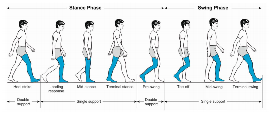
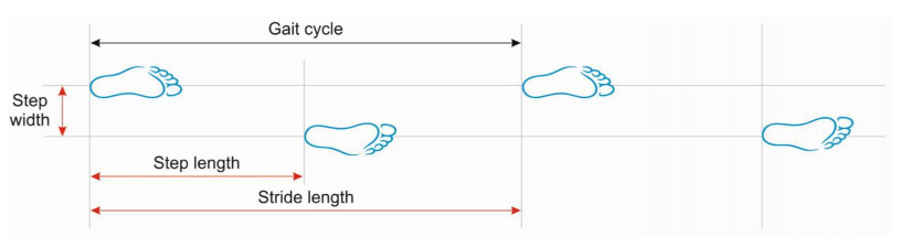
🔎 Gait disorders in adults and the elderly.
phases of a walking gait cycle
Pirker and Katzenschlager 2017.
P4
Walking VS Running
| Walking | Running |
|---|---|
 Walking: move without loss of contact, or flight phases | 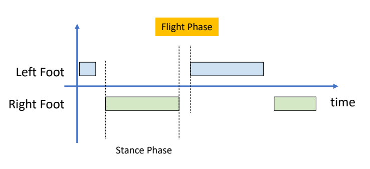 |
P7
Walking的几个阶段
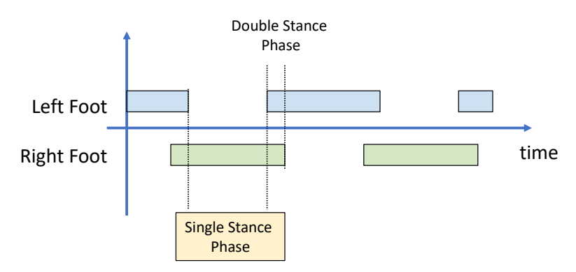 | 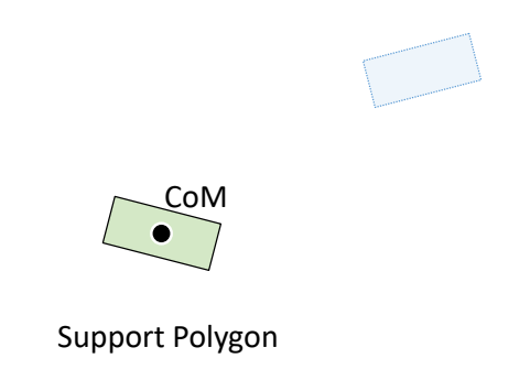 |
 | 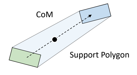 |
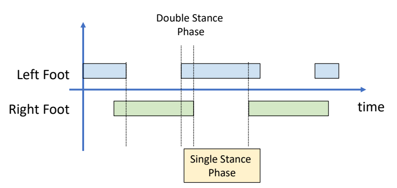 | 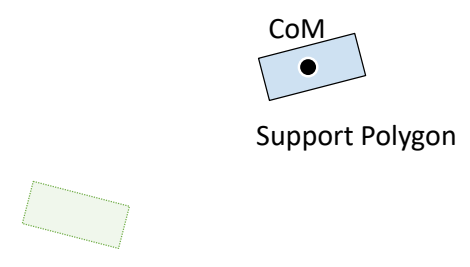 |
✅ 以上过程假设角色处于 static 状态。没有考虑到移动过程中的脚的动量。因此只能勉强保持角色稳定。要以非常慢的速度相前移动。
本文出自CaterpillarStudyGroup,转载请注明出处。
https://caterpillarstudygroup.github.io/GAMES105_mdbook/
P11
Zero-Moment Point (ZMP)
✅ 通过ZMP的控制实现比较稳定的走路。
全身受力分析与问题简化
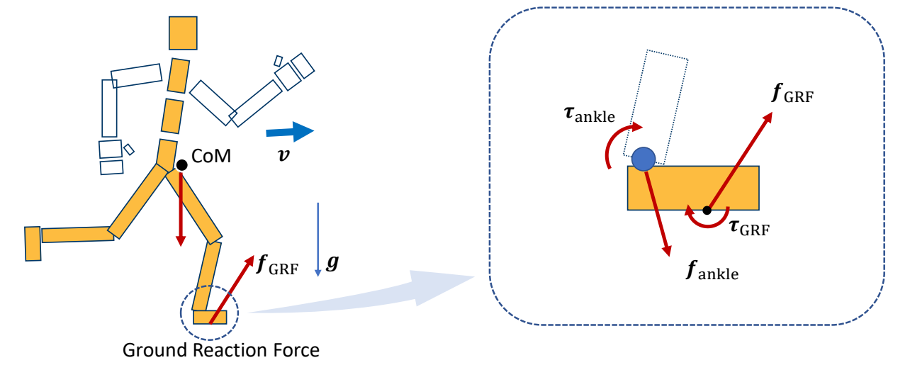
✅ 角色受到重力和GRF力。
✅ GRF = 支持力(向上)+ 动摩擦力(有速度时才有)
✅ 简化:上半身受到的所有的力,都体现在 ankle 关节上。
✅ 通过对 ankle 施加力/力矩来实现全身移动。
P12
Recall: A System of Links and Joints
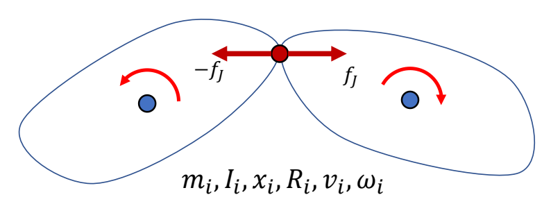
$$ M\dot{v} +C(x,v)=f+f_J $$
✅ 在满足这个公式的前提下,一个部分动了另一个部分就会跟着动。因此可以把问题简化,只分析ankle。
P15
脚上受力分析
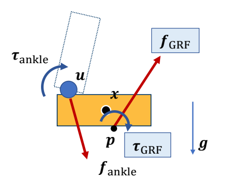
✅ 仅分析脚上的力,\(f_{\text{ankle}}\) 为 ankle 上的力转化到脚上的力。
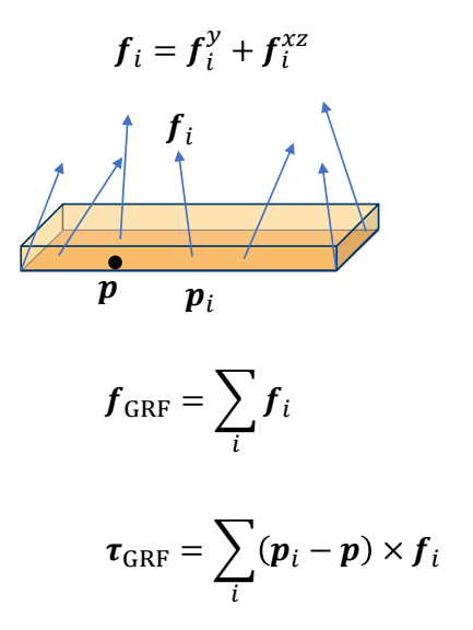
✅ 地面对脚的力不是施加到某一个点上,但可以根据公式换算成施加到某一点的力。
P17
Assuming the ground is flat and level
so \(p_i\) - \(p\) is always in the horizontal plane
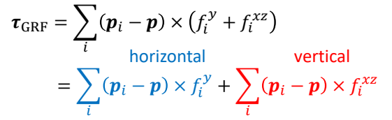
✅ 把 \(\tau _{GRF} \) 分解为与地面垂直部分和与地面平行部分(力矩的方向是指它的旋转轴的方向。),其中垂直的部分为:
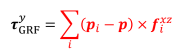
水平的部分为:
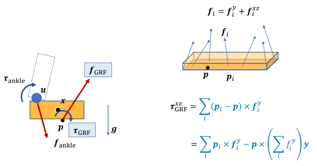
Can we find \(p\) such that \(\tau _{GRF}^{xz}=0\) ?
P21
Zero-Moment Point (ZMP)
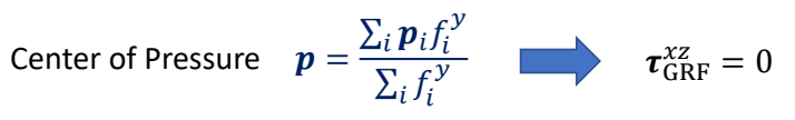
当\(p\) 为 center pressure时:
$$ \begin{align*} f_{GRF} & =\sum _{i}^{} f_i \\ \tau _{GRF} & =\tau _{GRF}^y=\sum _{i}^{}(p_i-p)\times f_i^{xz} \end{align*} $$
The position of \(p\) is not known, but we assume 以上公式成立。
ZMP条件下支撑脚的受力分析
假设: 支撑脚 should not move in a stance phase,且支撑脚与地面完成接触
则:在所有力作用下处于静平衡状态。
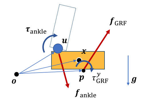
Static Equilibrium:
静态平衡满足:所有合力为0
$$
f_{\text{ankle}} + f_{\text{GRF}} + mg = 0
$$
静态平衡满足:任选一个参考点,所有合力(力矩)相对于参考点的动量为0,否则会旋转。
The moment around a reference point \(o\):
$$ (u-o) \times f_{\text{ankle}} + (p-o) \times f_{\text{GRF}} + (x-o)\times mg + \tau _{GRF}^{y} + \tau _{\text{ankle}} = 0 $$
✅ \(o\) 是一个参考点,可以在任意位置
✅ U:ankle 位置。
✅ X:质心位置 ✅ P:位置未知,高度为 0.
同样只关心水平方向:
Horizontal components (moment projected onto \(xz\) plane):
$$ ((u-o) \times f_{\text{ankle}})^{xz} +( (p-o) \times f_{\text{GRF}} ) ^{xz}+ (x-o)\times mg + \tau _{\text{ankle}}^{xz} = 0 $$
✅ 总力矩为 0,否则人会旋转。
P28
求解 Zero-Moment Point (ZMP)
We can solve this equation to find \(p\)
\(p\) is called Zero-Moment Point (ZMP) because it makes
$$ \tau _{GRF}^{xz}=0 $$
and the horizontal moment
$$ ((u-o) \times f_{\text{ankle}})^{xz} +( (p-o) \times f_{\text{GRF}} ) ^{xz}+ (x-o)\times mg + \tau _{\text{ankle}}^{xz} = 0 $$
Only when 𝑝 is within the support polygon!
✅ \(p\) 满足(1)水平力矩为0. (2)人整体上平衡。
✅ \(u,O,X\) 都是已知,\(p\) 的高度为 0,只有 \(P_xP_y\) 未知且该公式分别在 \(X\) 和 \(Z\) 上成立,实际上是两个方程。
✅ 两个未知量和两个方程,可以解出 \(p\)。
P33
如果解出公式得到的\(p\) is outside the support polygon,那么:
\(p\) could NOT be the center of pressure, because all the GRFs
are applied within the polygon, so that
$$ \tau _{GRF}^{xz}\ne 0 $$
✅ 如果求出 \(p\) 在 polygon外 则不能平衡,因为不是 center pressure.
如果选择polygon上的real center of pressure\({p}' \) ,那么:
$$ ((u-o) \times f_{\text{ankle}})^{xz} +( ({p}'-o) \times f_{\text{GRF}} ) ^{xz}+ (x-o)\times mg + \tau _{\text{ankle}}^{xz} \ne 0 $$
✅ \({p}' \ne p\),\({p}'\) 处水平方向的合外力不为零,脚会翻转人会摔倒。
Simplified Models
P35
关于ZMP的思考
The existence of ZMP is an indication of dynamic balance We can achieve balanced walking by controlling ZMP But how?
P36
Simplified Models的基本套路
- Simplify humanoid / biped robot into an abstract model
- Often consists of a CoM and a massless mechanism
- Need to map the state of the robot to the abstract model
✅ 因此,把最影响平衡的量拿出来,建立简化模型。
✅ 实际上更加复杂,对上半身任何一个部位的干挠,都会影响到脚上的力。
-
Plan the control and movement of the model
- Optimization
- Dynamic programming
- Optimal control
- MPC
-
Track the planned motion of the abstract model
- Inverse Kinematics
- Inverse Dynamics
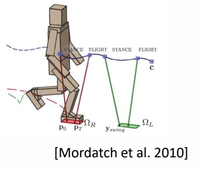
P37
Example: ZMP-Guided Control
🔎
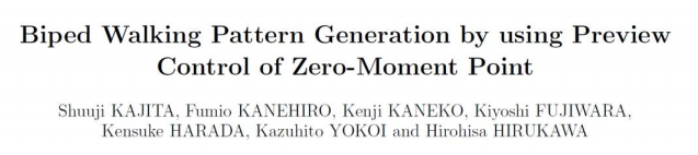
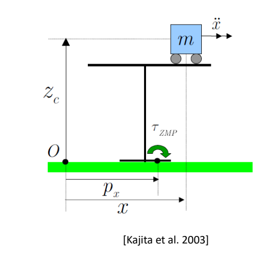
✅ 把机器人简化为桌子和小车,通过控制小车m的运动来控制 ZMP。使 ZMP 满足预定义轨迹。
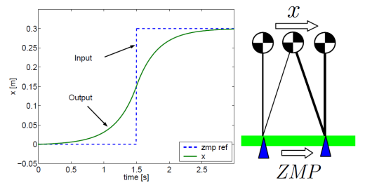
✅ 预定义轨迹的轨迹是指保持在pologon里面。通过优化得到 \(m\) 的运动。
✅ 然后通过IK和PD control控制脚的运动。
✅ ASIMO机器人局限性:(1) 脚必须与地面平行。 (2) 脚必须弯曲。 (3) 整体移动速度慢。
P40
Inverted Pendulum Model (IPM)
Walking == Falling + Step Planning
✅ 人的特点是重心偏离再拉回来,这样比始终保持平更省。
P42
IPM问题
✅ IPM: 倒立摆模型,控制小车使杆不掉下去。
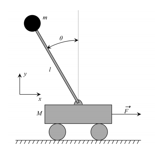
Step Plan with IPM
🔎

P45
- Map CoM of the character and the stance foot as IPM
- Plan the position of the next foot step so that the mass point rests at the top of the pendulum
- Create foot trajectory based on the step plan
- Compute target poses using IK
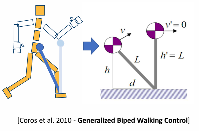
✅ 脚到重心是一个倒立摆。
✅ 由于失去平衡,质心有一个向前的速度,通过到一个合适的落脚点,使质心到达脚的正上方刚好到达速度稳定。
✅ 算出脚的目标位置后,插值,IK,PD 控制。
P46
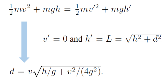
✅ 动能转势能,能量守恒.算出高度。
❗ 注意:杆的长度是不确定的,因为腿会弯曲。
P47
✅ 方法优点:可以适用于不同角色,不同动作,不同环境交互。
本文出自CaterpillarStudyGroup,转载请注明出处。
https://caterpillarstudygroup.github.io/GAMES105_mdbook/
P48
SIMBICON
🔎 SIMBICON (SIMple BIped Locomotion CONtrol) Yin et al. 2007
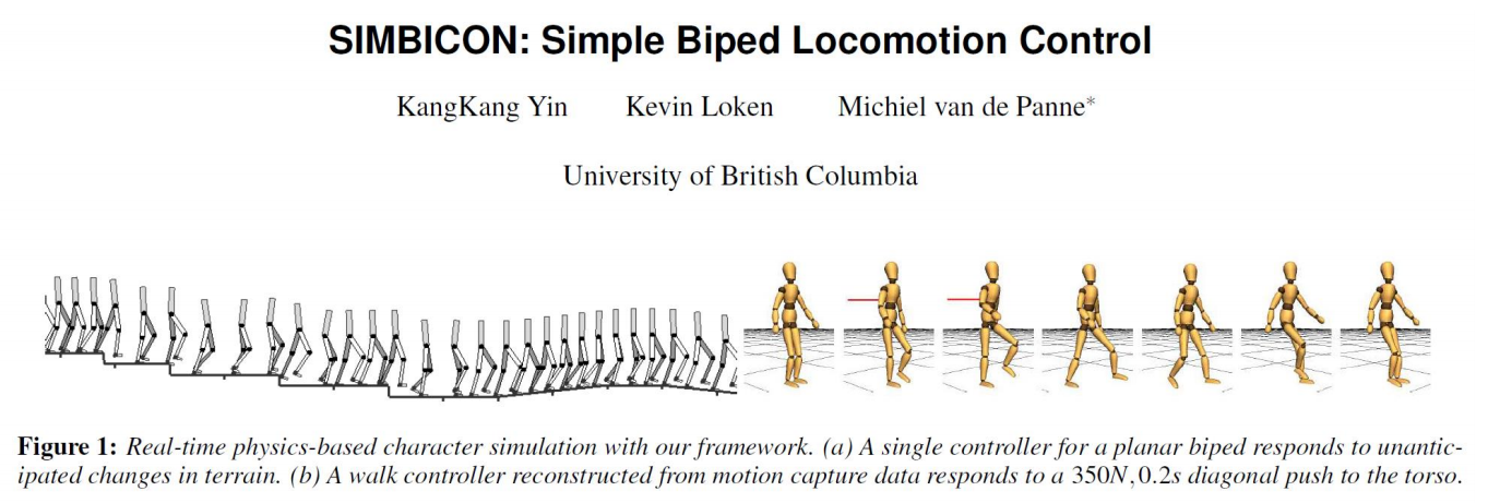
✅ 经典工作,第一个实现了鲁棒的步态控制。
✅ 原理:跟踪控制器上加一个反馈
P49
Step 1
- Step 1: develop a cyclical base motion
- PD controllers track target angles
- FSM (Finite State Machine) or mocap
✅ 本质上是一个跟踪控制器,用状态机来实现的跟踪控制器
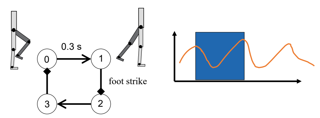
✅ 有四个状态,通过跟踪在4个状态之间切换,也可以用动捕数据来代替
P50
Step 2
- Step 2:
- control torso and swing-hip wrt world frame
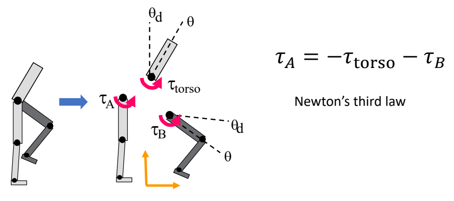
✅ 控制目标:上半身保持竖直。
✅ 控制方法:
通过保持上半身竖直,计算出\(\tau _{\text{torso}} \)。
通过使B跟踪目标动作,计算出\(\tau _{B} \)。
通过 \(\tau _{\text{torso}} \) 和 \(\tau _{B} \) 控制 \(\tau _{A} \).
P51
Step 3
- Step 3: COM feedback
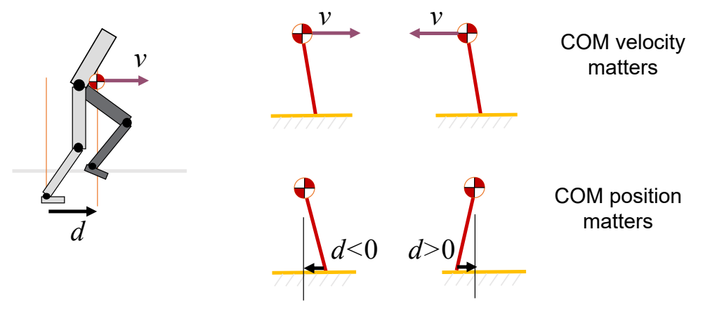
✅ 估计下一个脚步的位置d,使质心处于可控范围内。
✅ \(d\) 与 \(D\) 有关,但关系复杂,在此处做了简化。
P52
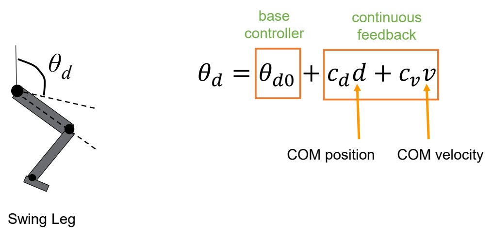
✅ 简化问题:\(d\) 和 \(v\) 与 \(\theta _d\) 的速度是线性关系。速度会转化为 PD 目标的修正。
✅ 线性的系数为手调。
P53
SIMBICON
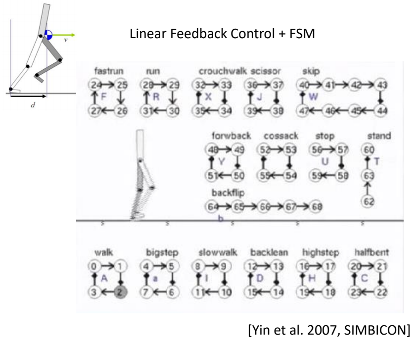
P54
Outline
- How to generalize to other motion?

本文出自CaterpillarStudyGroup,转载请注明出处。
https://caterpillarstudygroup.github.io/GAMES105_mdbook/
混合方法
✅ 本章定位:理解如何在动力学方法中引入运动学数据,实现高质量且符合物理的角色动画。
运动学 vs 动力学:优缺点对比
运动学方法
优点:
- 动作质量高:来自动捕数据,真实自然
- 计算效率高:无需物理仿真,实时性好
- 易于控制:直接输出姿态,可控性强
缺点:
- 不符合物理:穿模、滑步、浮空
- 抗扰动能力差:受外力后无法恢复
- 无法与环境交互:不能适应地形变化
动力学方法
优点:
- 符合物理:无穿模、滑步
- 抗扰动能力强:受外力后可恢复平衡
- 可与环境交互:适应地形、物体交互
缺点:
- 动作质量低:像机器人、僵硬
- 计算成本高:需要物理仿真、优化/训练
- 调参困难:需要大量手工调整
为什么要结合?
核心思想:取长补短
┌─────────────────────┐     ┌─────────────────────┐
│   运动学方法        │     │   动力学方法        │
│                     │     │                     │
│  ✓ 动作质量高       │     │  ✓ 物理真实         │
│  ✓ 计算效率高       │     │  ✓ 抗扰动强         │
│  ✓ 易于控制         │     │  ✓ 可交互           │
│                     │     │                     │
│  ✗ 不符合物理       │     │  ✗ 动作质量低       │
│  ✗ 抗扰动差         │     │  ✗ 计算成本高       │
│  ✗ 无法交互         │     │  ✗ 调参困难         │
└─────────────────────┘     └─────────────────────┘
            ↓                           ↓
            └──────────┬────────────────┘
                       │
                       ↓
            ┌─────────────────────┐
            │    混合方法         │
            │                     │
            │  ✓ 动作质量高       │
            │  ✓ 物理真实         │
            │  ✓ 抗扰动强         │
            │                     │
            │  ✗ 系统复杂         │
            │  ✗ 训练成本高       │
            └─────────────────────┘
混合方法的本质
┌─────────────────────────────────────────────────────────┐
│  混合方法 = 动力学方法 + 运动学数据                      │
│                                                         │
│  动力学方法提供:物理仿真、抗扰动能力                    │
│  运动学数据提供:高质量动作参考、风格先验                │
└─────────────────────────────────────────────────────────┘
与前面章节的关系:
运动学方法 ──→ 提供数据/先验 ──┐
                              ├──→ 混合方法
动力学方法 ──→ 提供仿真/执行 ──┘
常见的结合套路
套路 1:先运动学,后动力学(串联)
运动学生成初值 → 动力学优化 → 输出
代表:DReCon(Motion Matching + 轨迹优化)
流程:
- Motion Matching 从数据库中找到最匹配的 pose 作为初值
- 轨迹优化在初值基础上做物理适配
- PD 控制执行
优点:动作质量高,物理真实 缺点:系统复杂,需要维护数据库
套路 2:运动学指导动力学生成(并行)
运动学数据 → 学习先验 ──┐
                        ├──→ 动力学方法生成
动力学方法 ─────────────┘
代表:AMP(对抗式运动先验)
流程:
- 用动捕数据训练判别器(学习风格先验)
- RL 策略生成动作,判别器判断"像不像"
- 策略不断优化,生成既符合物理又像动捕风格的动作
优点:推理时无需参考数据,可泛化 缺点:训练成本高,需要大量采样
套路 3:运动学作为跟踪目标(强耦合)
运动学轨迹 → 目标 → 动力学跟踪
代表:DeepMimic
流程:
- 动捕轨迹作为参考目标
- RL 学习如何跟踪参考轨迹
- 跟踪策略输出关节力矩,通过仿真器执行
优点:动作质量高,抗扰动 缺点:推理时仍需参考轨迹,泛化能力有限
套路 4:端到端学习(隐式结合)
状态输入 → 神经网络 → 力矩/姿态输出
           (训练时用了运动学数据)
代表:UniPhys、CAMDM(Diffusion 模型)
流程:
- 用动捕数据(状态 - 动作对)训练模型
- 模型直接输出力矩或姿态
- 端到端,无需手动设计接口
优点:系统简单,推理快 缺点:需要大量训练数据,可解释性差
与前面章节的关系
四种套路的对比
| 套路 | 代表方法 | 运动学数据形式 | 动力学方法 | 依赖程度 |
|---|---|---|---|---|
| 串联 | DReCon | 动作数据库 | 轨迹优化 | 中 |
| 并行 | AMP | 风格先验 | RL 生成 | 弱 |
| 强耦合 | DeepMimic | 完整轨迹 | RL 跟踪 | 强 |
| 端到端 | UniPhys | 状态 - 动作对 | Diffusion 策略 | 中 |
深入学习:DeepMimic | AMP | DReCon | UniPhys
与前面章节的关系
| 章节 | 与混合方法的关系 |
|---|---|
| 轨迹优化 | 混合方法可以借用轨迹优化进行物理适配 |
| 角色控制 | 混合方法可以看作"有数据引导的角色控制" |
| PD 控制 | 混合方法的输出通常通过 PD 控制执行 |
本章重点问题
-
如何设计运动学数据与动力学方法的接口?
- DeepMimic:参考轨迹作为 reward
- AMP:动捕数据训练判别器
- DReCon:数据库提供初值
-
如何平衡数据依赖与泛化能力?
- 强依赖:动作质量高,但泛化差
- 弱依赖:泛化好,但训练难
-
如何处理训练与推理的差异?
- 训练时:可以用动捕数据
- 推理时:根据方法不同,依赖程度不同
深入学习:ReadPapers - Physics-based Character Control
Locomotion
任务:实时控制虚拟角色进行高效、真实、可控且自适应的行走、奔跑、跳跃等基础位移运动。
mindmap
    Locomotion
        多
            更多的动作类型
                适配不同地形(平地、楼梯、斜坡)
                适配不同角色
                    二足/四足
                    不同体型
                不同的动作
                不同的风格
            更多的应用场景
                路径引导
                风格控制
                动作类型切换
                动作插帧
                实时运动输入(如动捕、VR 追踪数据)
        快
            满足交互式场景的帧率要求
            快速地数据准备
        好
            动作具有物理真实感
                运动轨迹、肢体姿态、步态节奏符合生物力学规律
                无穿模、僵硬、浮空等失真现象
            动作具有生物真实感
                还原人类 / 生物自然运动特征
            符合用户控制
                支持用户高层指令(速度、方向、动作风格、启停)的精准响应
                实现细粒度运动调节
            稳定性
                具备外力扰动下的稳定性
        省
            计算开销低
            更少的数据
            更少的人工参与
            更少的预处理
                在适配不同泛化性问题时,无需重新设计运动逻辑
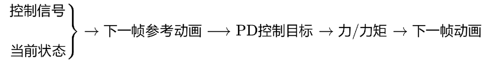
直接使用“下一帧参考动画”作为角色动作数据的方法称为基于运动学的方法。 由力/力矩产生的“下一帧动画”作为角色动作数据的方法称为基于动力学的方法。
mindmap
Locomotion
    基于运动学
        数据库匹配
            状态机
            动作匹配
        监督学习
            基于相位
            不基于相位
        生成模型
            基于当前帧的生成 + <br>结合控制目标的策略
            diffusion
    基于动力学
         目标优化
         策略优化
基于运动学的方法:直接控制每个关节的动画数据,不考虑其物理合理性,其效果上限受制于数据。
基于动力学的方法:不直接提供动画数据,而是提供关节受力,让每个关节在力的作用下运动。
说明:
- 轨迹跟踪:下一帧参考动画 → 下一帧动画
- 轨迹优化:下一帧参考动画 → PD控制目标
实际的动力学算出过程,不一定会显式地出现每个步骤,可能是几个步骤统一到一个步骤中的。
基于匹配的方法
graph TD
    A[当前帧 frame] --> B{是否匹配?}
    B -- N --> C[下一帧 frame]
    B -- Y --> D[提取特征]
    D --> E[当前特征]
    F[获取数据] --> D
    G["(5) 角色状态"] --> D
    D --> H[最近邻搜索]
    H --> I[当前帧 frame]
    J[控制目标] --> H
    H --> K["(3) 下一帧动作"]
    L["(6) 角色的动作数据集"] --> M[提取特征]
    M --> N[特征集]
| ID | Year | Title | 特点 |
|---|---|---|---|
| - | - | Motion Field | - |
| - | - | Motion Graph | Baseline,以 clip 为单位 (1) 只在一个 clip 结束时重新匹配 (2) 寻找最像的 clip,并用插值衔接 |
| - | - | Motion Matching | 以 frame 为单位 (1) 每帧或几帧重新匹配,响应更快 (2) 寻找最近匹配的帧,并用 blend 衔接 |
| - | 2020 | Learned Motion Matching | 基于数据集,把 (1)(2)(3) 替换成了网络模块,消除了在线搜索时对数据库的依赖 |
| P47 | Ⓐ | (风格迁移) | 让 (5) 和 (6) 分别是不同的角色,并增加将运动内容与运动风格解耦的模块。在运动空间进行最近邻匹配,在匹配空间中融入目标风格,实现在线风格迁移的效果。 |
Motion Graph / Motion Matching / Motion Field
flowchart LR
A([当前帧frame]) --> B("是否重新匹配(1)")
    B -->|"N"|C([当前帧frame])
    C --> D["(3)取下一帧动作"]
    D --> E([下一帧frame])
    E --> A
    F --> G(["(5)角色状态"])
    H([控制目标])
    G --> I["(4)提取特征"]
    H --> I
    I --> N([当前特征])
    N -->J["(2)最近邻搜索"]
    J -->C
    B --> F["(5)取数据"]
    K(["(6)角色的动作数据集"])
    K --> L["(4)<br>提取特征"]
    L --> M(["特征集"])
    M --> J
    K --> D
| ID | Year | Title | 特点 |
|---|---|---|---|
| Motion Field | |||
| Motion Graph | Baseline,以clip为单位 (1) 只在一个clip结束时重新匹配自己 (2) 寻找最适配的clip,并用拖帧衔接。 | ||
| Motion Matching | 以frame为单位 (1) 每帧或几帧重新匹配,响应更快 (2) 寻找最匹配的帧,并用blend 做衔接。 | ||
| - | 2020 | Learned Motion Matching | 基于数据集,把 (1)(2)(3)(4) 替换成了网络模块,消除了在线推理时对数据库的依赖。 |
| 209 | 2023.10.16 | MOCHA: Real-Time Motion Characterization via Context Matching | 让 (5) 和 (6) 分别是不同的角色,并增加将运动内容与运动风格解耦的模块。 在运动空间进行最近邻匹配,在匹配结果中融入目标风格,实现在线风格迁移的效果。 |
通过检索、拼接、插值实现运动生成,是工业界长期主流方案。
优势:
- 实现简单:基于准备好的数据库,即可以与角色进行实时控制
- 可控性高
缺点:
- 依赖特定角色的海量数据
- 最近邻搜索成本高
- 内存占用大
- 对不同地形泛化性差
- 随着数据集规模增大,扩展性较差
基于监督学习的方法
非相位方法
| ID | Year | Name | 解决了什么痛点 | 主要贡献是什么 | Tags | Link |
|---|---|---|---|---|---|---|
| 2018.10.4 | Recurrent Transition Networks for Character Locomotion | 传统方法(如运动图、高斯过程模型)存在泛化性差、仅适配单一动作类型、运行时计算成本高等问题。 基于深度学习的“从当前状态到目标状态的定向过渡生成”处于研究空白 | 1. 改进型 LSTM:传统 LSTM 仅依赖历史状态,RTN 在门控计算中加入未来上下文特征(目标 + 偏移),使生成过程始终朝向目标状态,避免无约束漂移; 2. 隐藏状态初始化:摒弃 “零向量初始化” 或 “全局共享初始状态”,通过 MLP 学习输入首帧与最优初始隐藏状态的映射,让 LSTM 从初始阶段就捕捉运动特征,提升生成质量; 3. ResNet 风格解码器:输出当前帧与下一帧的偏移量,而非直接输出姿态,减少生成帧与输入上下文的间隙,提升过渡流畅性。 | link |
基于相位的方法
flowchart LR
    C([NN2])-->A
    D([NN3]) -->A
    E([NN4]) -->A
    B([NN1]) -->A[专家混合]
    A-->F([混合专家模型])
    F-->G[模型推理]
    H(["控制目标<br>(轨迹、标签)"])-->G
    J([当前状态])-->G
    G -->K([相位变化量])-->P([相位])-->O([当前相位])
    G -->L([触地信息])-->R[IK]-->N
    G -->Q([未来轨迹])-->N
    G -->M([下一帧状态])-->N([动作输出])-->J
    O -->A
优势:
- 能对用户输入做出稳定实时的响应。
局限性:
- 依赖精心的设计
- 用高度可变的运动数据进行训练,会产生平均化的结果。
- 难以泛化到数据以外的动作。
| ID | Year | Name | 解决了什么痛点 | 主要贡献是什么 | Tags | Link |
|---|---|---|---|---|---|---|
| 212 | 2023.8.24 | Motion In-Betweening with Phase Manifolds | 首次将周期自编码学习的相位流形引入角色补间动画 | 1. 将复杂的人体运动分解到频域,用相位 + 振幅编码运动的周期性和时序规律。 2. 相位提取:DeepPhase. 3. 双向控制:角色坐标系 + 目标坐标系。 4. 用户控制:轨迹控制、动作类型控制。 | 多:超长动作插帧 快:实时动作插帧 好:可进行路径、风格控制 | |
| 211 | 2022.1.12 | Real-Time Style Modelling of Human Locomotion via Feature-Wise Transformations and Local Motion Phases | 将相位方法引入到风格迁移任务中。 | 1. 发布了 100 style 数据集 2. 扩展相位提取方式,对于非接触运动也能提取相位:对同一类数据使用 PCA 提取主成分,取第一主成分的系数。若存在周期性,用 sin 函数拟合系数。 3. 注入风格:输入风格 clip,输出 alpha 和 beta,用于调制主网络的隐藏层。训练时,先训练主网络,再接入 FiLM,并 finetune FiLM。推断时,不需要 FiLM,使用预置风格的 alpha 和 beta,也可以用插值得到 alpha 和 beta。 | 多:具有风格迁移能力。动作泛化到非接触的周期动作。 快:实时的风格切换。 好:连续的风格参数,风格切换无跳变。 | |
| 211 | 2020.7.8 | Local Motion Phases for Learning Multi-Contact Character Movements | 1. PFNN 只用于周期性动作; PFNN 需要手动标注相位 | 1. 非周期动作=各个局部周期动作的叠加,因此给几个重要的关节独立的相位。 2. 自动提取相位的方法:定义接触为 1,再用 sin 函数拟合。 3. 一个权重估计网络,输入 n 个相位,输出 m 个权重参数。 4. 用户的控制信号过于稀疏,导致生成结果平均化。因此训练生成模型 GAN,根据稀疏控制信号生成细节控制信号。 | 多:泛化到非周期动作。 好:引入生成模型,避免动作趋于平均化。 省:无须人工标注。 | |
| 214 | 2018.10.1 | Few-shot Learning of Homogeneous Human Locomotion Styles | 小样本的学习策略 | 1. 数据准备:(1) 大量基本风格数据(2)少量特定风格数据 2. 模型准备:用 PFNN 实现通用模块,用 residual adapter 来实现 style 模块 3. 训练策略:数据(1)用于通用模块与 style 模块的解耦,数据 (2) 用于 finetune style 模块 4. 参数策略:将 adapter 矩阵分解为 X=ADB^T,进一步减少参数量。 | 多:泛化到不同风格。 快:少量样本即可迁移,训练快。 好:无过拟合,泛化性好。 少:省训练数据,少内存。 | |
| 213 | 2018.6.30 | Mode-Adaptive Neural Networks for Quadruped Motion Control | 传统数据驱动方法(运动图、运动匹配):需存储完整动作数据库,依赖手动分割、标注,搜索过程复杂,实时性差;CNN 存在输入输出映射模糊问题,RNN 长期预测易收敛到平均姿态(漂浮),PFNN 虽解决模糊问题,但依赖手动相位标注,无法适配非循环运动。 | 本文提出模式自适应神经网络(MANN),专为四足动物运动控制设计,核心通过"门控网络 + 运动预测网络"的双模块架构,从大规模非结构化动作捕捉(MOCAP)数据中自主学习运动模式,无需手动标注相位或步态标签;门控网络基于脚部关节速度、目标速度等特征动态加权多个专家网络输出,运动预测网络生成平滑连贯的下一帧运动,支持怠速、移动、跳跃、坐姿等多种循环与非循环运动,同时允许用户通过速度、方向、动作变量交互控制。 | PPT | |
| 113 | 2017.7.20 | Phase-functioned neural networks for character control | 1. Motion Matching 需要存储大量数据 2. 自回归方法存在误差积累 3. CNN方法不能实时 4. 物理方法不可控 5. 不能支持复杂地形 | 1. 混合专家模型,首次将运动相位从「网络输入特征」升级为「网络权重的全局参数化变量」2. 将平地动捕数据与复杂地形耦合,让模型学会了根据地形自动调整动作。 Baseline | PFNN 多:支持不同地形的泛化性 快:0.8ms/帧 好:1. 混合专家模型,解决相位混合引入的artifacts 2. IK后处理解决脚本问题 省:引入NN,不需要存储原始数据 | link |
基于生成的方法
生成 + 控制
(1) 无控制自回归生成模型
flowchart LR
 A([数据集])-->|"预训练"|C[先验模型]
 B([当前状态])--> C-->D([下一帧状态])
(2) 引入控制策略
flowchart LR
 A([控制目标])-->B([策略])--> D[先验模型]--> E([下一帧状态])
 C([当前状态])--> D
flowchart LR
 A([当前状态])-->B[先验模型]
 B--> C([生成1])--> F
 B--> D([生成2])--> F
 B--> E([⋮])--> F
 B--> G([生成n])--> F
 F([选出下一帧])
| ID | Year | Title | 特点 |
|---|---|---|---|
| 136 | 2021.3.26 | Character Controllers Using Motion VAEs | 在给定足够丰富的运动捕捉片段集合的情况下,如何实现有目的性且逼真的人体运动 |
| 206 | 2024.8.16 | Interactive Character Control with Auto-Regressive Motion Diffusion Models (A-MDM) | A-MDM 136 中的 VAE 替换成了 MLP diffusion 并使用分层强化学习进行控制。 |
条件生成
flowchart LR
 A([当前状态])--> C
 B([控制目标])--> C
 C([条件])--> F[Diffusion]--> G([latent code]) --> H[Decoder]--> I([下一帧状态])
 D([噪声])--> F
 E([t])-->F
- 难以在各种控制信号间进行泛化。
- 难以泛化到数据以外的动作。
- 支持多模态条件信号和任意损失引导。
- 能够实现更长期的目标和复杂任务。
| ID | Year | Name | 解决了什么痛点 | 主要贡献是什么 | Tags | Link |
|---|---|---|---|---|---|---|
| 187 | 2025.5.30 | MotionPersona: Characteristics-aware Locomotion Control | 首个生成式角色控制器。实时交互 + 角色个性化 | 1. 输入:文本描述->CLIP->emb,SMPL beta,历史状态,未来轨迹,示例版本 (Optimal) 2. 模型:DiT 结构,每次 45 帧,单帧>60fps 3. 动作衔接:在噪声空间对生成的前 5 帧与最后一帧做平滑 4. 推理时基于对小样本对编码层和输出层微调(DreamBooth) 5. 数据集 | 多:个性化 快:实时推理 省:极少的定制化数据及微调时间 | |
| 205 | 2025.5.13 | DARTControl: A Diffusion-based Autoregressive Motion Model for Real-time Text-driven Motion Control | 自然语言的角色控制,条件为自然语言。 为了支持轨迹控制,额外引入控制方式,类似上文“生成 + 控制”方法。 | link | ||
| 204 | 2024.7.11 | AAMDM: Accelerated Auto-regressive Motion Diffusion Model | 使用 DDGAN 进行推断加速 | link | ||
| 177 | 2024.4.23 | Taming Diffusion Probabilistic Models for Character Control (CAMDM) | 这篇发表于 SIGGRAPH 2024 的论文聚焦基于扩散模型的实时角色控制,提出了条件自回归运动扩散模型(CAMDM),首次将运动扩散概率模型成功落地到实时交互式角色控制场景中。核心解决了传统扩散模型计算量大、可控性差、多样性不足的问题,实现了单模型支持多风格、实时响应用户控制、生成高质量且多样化的角色动画,同时能完成风格间的无缝过渡,是角色动画和运动生成领域的重要突破。 |
基于动力学的方法
核心特征:输出为关节力矩或 PD 控制目标,需要物理仿真器执行。
与运动学方法的区别:
| 维度 | 运动学方法 | 动力学方法 |
|---|---|---|
| 输出 | 关节姿态/速度 | 关节力矩/PD 控制目标 |
| 物理仿真 | 否 | 是 |
| 抗扰动能力 | 无 | 有 |
| 训练成本 | 低 | 高 |
| 实时性 | 高 | 中 |
mindmap
基于动力学的方法
    参考学习
        运动生成 + 运动模仿/sim2real
        运动先验 + 下游控制
    无参考的强化学习
        设计规则作为先验
        纯强化学习无先验
无参考的强化学习
优势:
(1) 能够生成新颖且符合物理规律的动作
(2) 数据依赖少
局限性:
(1) 开销问题
(2) 可扩展性问题
(3) 需要大量手工调优奖励函数,收敛速度慢,在步态切换、跳跃等复杂机动动作上难以实现稳定表现。
| ID | Year | Name | 解决了什么痛点 | 主要贡献是什么 | Tags | Link |
|---|---|---|---|---|---|---|
| 2007.7.29 | SIMBICON: simple biped locomotion control | ① 零力矩点(ZMP)方法依赖预计算轨迹,灵活性不足; ② 强化学习 / 策略搜索需设计复杂奖励函数,高维状态下难以收敛; ③ 数据驱动方法多为运动学建模,缺乏物理适应性。 | “有限状态机 + 全局坐标控制 + 质心反馈” 的极简组合,无需复杂动力学建模,实现实时、鲁棒的物理基双足运动生成 | link |
| ID | Paper | Note |
|---|---|---|
| 185 | Gait-Conditioned Reinforcement Learning with Multi-Phase Curriculum for Humanoid Locomotion | 1. 单个循环策略同时学习站立、行走、奔跑及步态过渡,避免多策略架构的切换复杂度 2. 一种路由机制根据步态 ID 动态激活步态目标,核心解决不同步态的奖励目标冲突问题 3.让机器人自主学习符合人体生物力学的自然运动,摆脱对 MoCap 数据的依赖 4. 用于技能扩展的渐近式多阶段课程。 |
基于参考的学习,例如APM、模仿学习,动作空间还是来自于数据,物理只是一种动作合理化的方法。 优势:
- 物理的方法与数据的方法相结合,利用两种范式的优势,提升运动质量、多样性的泛化能力。
局限性: - 依赖高质量数据
- 存在数据角色与被驱动角色之间的形态不匹配
- 难以泛化到数据分布之外
运动先验 + 下游控制
类似于“生成 + 控制”
- 每个任务都需要单独训练策略
| ID | Year | Name | 解决了什么痛点 | 主要贡献是什么 | Tags | Link |
|---|---|---|---|---|---|---|
| 198 | 2022.5.12 | AMP: Adversarial Motion Priors for Stylized Physics-Based Character Control | 模仿学习时,模仿目标需要精心设定,模仿效果的目标函数也难设定。 | 不模仿特定的动作,而是模仿目标动作的风格。通过对抗学习来判断模仿的风格像不像。 AMP 动作先验 = 对抗式判别器。 | link |
运动规划器 + 运动控制器 + 运动执行器(PD控制)
运动规划器:当前状态 + 控制目标 → 下一帧参考动画
运动控制器:下一帧参考动画 + 当前状态 → PD 控制目标
类似“可控生成 + 动作优化” 。
局限性:
- 规划器和控制器之间存在GAP,导致动作质量下降
- 控制策略难以准确跟踪规划的运动,需要微调,限制了其泛化能力
| ID | Paper | Note |
|---|---|---|
| 190 | DReCon: data-driven responsive control of physics-based characters | Motion Matching+RL 跟踪 +PD 执行 |
| 189 | PARC: Physics-based Augmentation with Reinforcement Learning for Character Controllers | 迭代数据扩增 |
| 188 | CLOSD: CLOSING THE LOOP BETWEEN SIMULATION AND DIFFUSION FOR MULTI-TASK CHARACTER CONTROL | Diffusion 规划器 +RL 跟踪器 |
(规划器, 控制器)+PD
由于规划器与控制器之间的 GAP,此文章开始尝试把它们统一到一个模型中
| ID | Paper | Note |
|---|---|---|
| 183 | Maskedmimic: Unified physics-based character control through masked motion | 掩码运动补全 |
| 192 | PDP: Physics-Based Character Animation via Diffusion Policy | RL 专家蒸馏 |
| 184 | UniPhys: Unified Planner and Controller with Diffusion for Flexible | 1. 把运动规划和控制整合到一个模型中,消除两个模型带来的 domaingap 2. 文本、目标、轨迹等多模态输入 3. Diffusion Forcing 范式进行训练,消除长期累计误差 4. 通过引导采样,无需 finetune,即可泛化到不同(包括没见过)的控制信号。 具体方法为行为克隆学习,先从动捕数据中提取状态 - 策略对,再用 diffusion 学习策略。 |
或者更直接一点,把PD也整合进一个模型,生成模型直接出力/力矩
| ID | Paper | Note |
|---|---|---|
| 186 | Diffuse-CLoC: Guided Diffusion for Physics-based Character Look-ahead | 直接生成力/力矩 |
控制 + 转移 + PD
与生成模型一样,数据也可以用于学状态转移,由RL来指导角色的控制性
| ID | Paper | Note |
|---|---|---|
| 191 | Universal Humanoid Motion Representations for Physics-Based Control | Prior+ 蒸馏 +RL |
运动执行器:
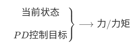
运动执行器可以是PD、PID等,图形学习里用的几乎都是PD。
所谓PD控制,实际不是控制器而是执行器。
PD控制器是传统方法,需要调 \(k_d\)、\(k_s\) 两个参数。用LQR可以计算出最能贴合目标的PD效果。
优点:
- 同“可控生成”
本文出自CaterpillarStudyGroup,转载请注明出处。
https://caterpillarstudygroup.github.io/GAMES105_mdbook/